Open Code in Cloud
Introduction
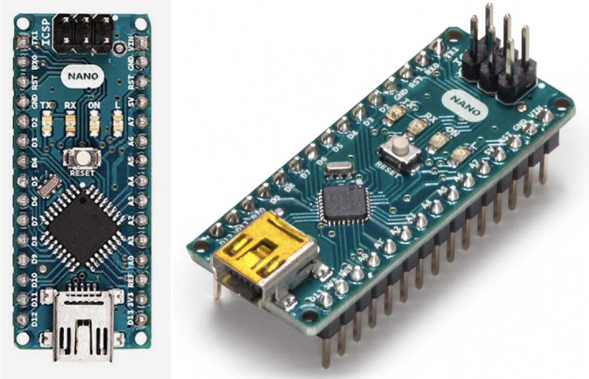
In this project I will analyze the responses of a bandpass Butterworth and Chebyshev1 filter deployed to an Arduino Nano from the Wolfram Language.
As these are analog filters, they need to be discretized before deployment. It is interesting to see in real-time how the frequency response of deployed filter closely matches that of the analog version.
The frequency responses create a mental imagery of what the real-time responses of the filters would look like and how they would differ from each other. But I wanted to make it concrete. So I created a visualization juxtaposing the frequency responses of the analog filters and the real-time responses of discretized filters, to see both in real-time as I change the parameters of the input signals.
In the first part, the filters are computed, analyzed, and deployed. In the second part, I acquire and analyze the filtered data to visualize the responses and evaluate the performance of the filters.
All the computations and tasks are done using the Wolfram Language: I use its signal processing capabilities to compute and analyze the filters, the Microcontroller Kit to deploy the filters, the device framework to do the data acquisition, and the notebook interface to visualize the data. If you are new to the Wolfram Language, there is a fast introduction that will quickly get you up to speed.
Compute, analyze, and deploy the filter
I start off by creating a function that will compute a filter with passband frequencies of 2 Hz and 5 Hz, stopband frequencies of 1 Hz and 10 Hz, and an attenuation of -30 dB at the stopband frequencies.
Clear[tfm]
tfm[filter_, s_: s] := filter[{"Bandpass", {1, 2, 5, 10.}, {30, 1}}, s] // TransferFunctionExpand // Chop
Using that I obtain the corresponding Butterworth and Chebyshev type 1 bandpass filters.
{brw, cbs} = tfm /@ {ButterworthFilterModel, Chebyshev1FilterModel};

Grid[{{"Butterworth filter", brw}, {"Chebyshev1 filter", cbs}},
 Background -> {None, {Lighter[#, 0.6] & /@ {cB, cC}}}, Frame -> True,
  Spacings -> {1, 1}, Alignment -> Left]
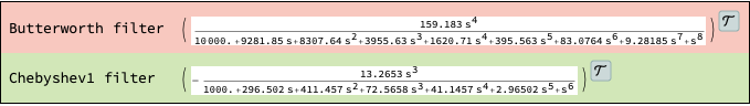
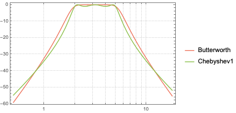
The Bode magnitude plot attests that frequencies between 2 Hz and 5 Hz are passed through, and frequencies outside this range are attenuated with an attenuation of around -35 dB at 1 Hz and 10 Hz.
{bMagPlot, bPhasePlot} =
  BodePlot[{brw, cbs}, {0.5, 18}, PlotLayout -> "List",
   GridLines -> Automatic, ImageSize -> Medium,
   PlotStyle -> {cB, cC, cI}, PlotTheme -> "Detailed",
   PlotLegends -> {"Butterworth", "Chebyshev1"}];

bMagPlot
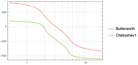
The phase plot shows that at around 3 Hz for the Butterworth filter and 2 Hz for the Chebyshev, there is no phase shift. For all other frequencies there are varying amounts of phase shifts.
bPhasePlot
Later I will put these frequency responses side by side with the filtered response from the microcontroller to check if they add up.
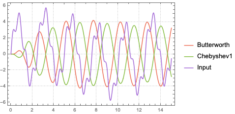
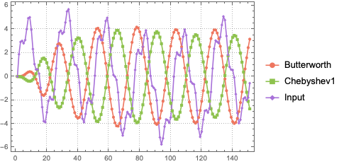
For now I will simulate the response of the filters to a signal with 3 frequency components. One component lies in the bandpass range and the other two lie outside it.
inpC = Sin[0.5 t] + 4 Sin[2.5 t] + Sin[10 t];
The responses show that the two frequences outside the bandpass are in fact stripped away.
outC = Table[OutputResponse[sys, inpC, {t, 0, 15}], {sys, {brw, cbs}}];
Plot[{outC, inpC}, {t, 0, 15},
 PlotLegends -> {"Butterworth", "Chebyshev1", "Input"},
 PlotStyle -> {cB, cC, cI}, PlotTheme -> "Detailed"]
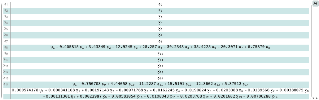
I then discretize the filters and put them together into one model.
sp = 0.1;

StateSpaceModel[ToDiscreteTimeModel[#, sp]] & /@ {brw, cbs} ;
sysD = NonlinearStateSpaceModel[
    SystemsModelParallelConnect[Sequence @@ %, {{1, 1}}, {}]] /.
   Times[1.`, v_] :> v // Chop
For good measure, I simulate and verify the response of the discretized model as well.
With[{tmax = 15}, With[{inpD = Table[inpC, {t, 0, tmax, sp}]},
  ListLinePlot[Join[OutputResponse[sysD, inpD], {inpD}],
   PlotLegends -> {"Butterworth", "Chebyshev1", "Input"},
   PlotStyle -> {cB, cC, cI}, PlotTheme -> "Detailed",
   PlotMarkers -> {Automatic, Scaled[0.025]}]]]
And I wrap up this first stage, by deploying the filter and setting up the Arduino to send and receive the signals over the serial pins.
? =
     MicrocontrollerEmbedCode[
      sysD, <|"Target" -> "ArduinoNano", "Inputs" -> "Serial",
       "Outputs" -> {"Serial", "Serial"}|>, "/dev/cu.usbserial-A106PX6Q"]
(The port name /dev/cu.usbserial-A106PX6Q will not work for you. If you are following along you will have to change it to the correct value. You can figure it out using DeviceManager on Windows, or by searching for file names of the form /dev/cu.usb* and /dev/ttyUSB* on Mac and Linux systems. )
At this point, I can connect any other serial device to send and receive the data. I will use device framework in Mathematica to do that, as its notebook interface provides a great way to visualize the data in realtime.
Acquire and display the data
To set up the data transfer, I begin by identifying the start, delimiter, and end bytes.
{sB, dB, eB} =
Lookup[?["Serial"], {"StartByte", "DelimiterByte",
"EndByte"}]
{19, 44, 17}
Then I create a scheduled task that, reads the filtered output signals and sends the input signal over to the Arduino, and runs at exactly the same sampling period as the discretized filters.
i1 = i2 = 1;
 yRaw = y1 = y2 = u1 = u2 = {};
task1 = ScheduledTask[
   If[DeviceExecute[dev, "SerialReadyQ"],
    If[i1 > len1, i1 = 1]; If[i2 > len2, i2 = 1];
    AppendTo[yRaw, DeviceReadBuffer[dev, "ReadTerminator" -> eB]];
    AppendTo[u1, in1[[i1++]]];
    AppendTo[u2, in2[[i2++]]];
    DeviceWrite[dev, sB];
    DeviceWrite[dev, ToString[Last[u1] + Last[u2]]];
    DeviceWrite[dev, eB]
    ]
   ,
   sp];
I also create a second and less frequent scheduled task that parses the data and discards the old values.
task2 = ScheduledTask[
   yRaw1 = yRaw;
   yRaw = Drop[yRaw, Length@yRaw1];
   {y1P, y2P} = Transpose[parseData /@ yRaw1];
   y1 = Join[y1, y1P];
   y2 = Join[y2, y2P];
   {u1, u2, y1, y2} = drop /@ {u1, u2, y1, y2};
   ,
   3 sp
   ];
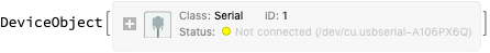
Now I am ready to actually send and receive the data, and I open a connection to the Arduino.
dev = DeviceOpen["Serial", "/dev/cu.usbserial-A106PX6Q"]
I then generate the input signals and submit the scheduled tasks to the kernel.
signals[w1, g1, w2, g2];
{taskObj1, taskObj2} = SessionSubmit /@ {task1, task2};
At this point, the data is going back and forth between my Mac and the Arduino. To visualize the data and control the input signals I create a panel. From the panel, I control the frequency and magnitude of the input signals. I plot the input and filtered signals, and also the frequency response of the filters. The frequency response plots have lines showing the expected magnitude and phase of the filtered signals, which I can verify on the signal plots.
DynamicModule[{iPart, ioPart,
  plotOpts = {ImageSize -> Medium, GridLines -> Automatic,
    Frame -> True, PlotTheme -> "Business"}}, Panel[Column[{

    Grid[{{
        Panel[Column[{
          Style["Input signal 1", Bold, cI1],
          Grid[{{"freq.",
             Slider[Dynamic[
               w1, {None, (w1 = #) &, signals[#, g1, w2, g2] &}], {0,
               7, 0.25}, Appearance -> "Labeled"]}}],

          Grid[{{"mag.",
             Slider[Dynamic[
               g1, {None, (g1 = #) &, signals[w1, #, w2, g2] &}], {0,
               5, 0.25}, Appearance -> "Labeled"]}}]}]]
       ,
       Panel[Column[{
          Style["Input signal 2", Bold, cI2],
          Grid[{{"freq.",
             Slider[Dynamic[
               w2, {None, (w2 = #) &, signals[w1, g1, #, g2] &}], {0,
               7, 0.25}, Appearance -> "Labeled"]}}],

          Grid[{{"mag.",
             Slider[Dynamic[
               g2, {None, (g2 = #) &, signals[w1, g1, w2, #] &}], {0,
               5, 0.25}, Appearance -> "Labeled"]}}]}]]
       }}
     ]

    ,
    Grid[{
      {
       Dynamic[
        ListLinePlot[{u1, u2, u1 + u2}[[iPart]],
         PlotStyle -> ({cI1, cI2, cI}[[iPart]]),
         PlotRange -> {All, (g1 + g2) {1, -1}}, plotOpts],
        TrackedSymbols :> {u1, u2},
        Initialization :> (iPart = {3}; g1 = g2 = 0;)]
       ,
       Dynamic[
        ListLinePlot[Join[{y1, y2}, {u1 + u2}][[ioPart]],
         PlotStyle -> ({cB, cC, cI}[[ioPart]]),
         PlotRange -> {All, (g1 + g2) {1, -1}},
         FrameTicks -> {{None, All}, {Automatic, Automatic}},
         plotOpts], TrackedSymbols :> {y1, y2, u1, u2},
        Initialization :> (ioPart = {1, 2})]
       }
      ,

      {
       Grid[{{CheckboxBar[Dynamic[iPart], Thread[Range[3] -> ""],
           Appearance -> "Vertical"], lI}}]
       ,
       Grid[{{CheckboxBar[Dynamic[ioPart], Thread[Range[3] -> ""],
           Appearance -> "Vertical"], lIO}}]
       }
      ,

      {
       Labeled[
        Dynamic[BodePlot[{brw, cbs}, {0.5, 18},
          PlotLayout -> "Magnitude", PlotLegends -> None,
          GridLines -> Automatic, ImageSize -> Medium,
          PlotStyle -> {cB, cC}, PlotTheme -> "Detailed",
          Epilog -> Join[mLine[w1, cI1], mLine[w2, cI2]]],
         TrackedSymbols :> {w1, w2}, SaveDefinitions -> True],
        "Bode magnitude"]
       ,
       Labeled[
        Dynamic[BodePlot[{brw, cbs}, {0.5, 18}, PlotLayout -> "Phase",
           PlotLegends -> None, GridLines -> Automatic,
          ImageSize -> Medium, PlotStyle -> {cB, cC},
          PlotTheme -> "Detailed",
          Epilog -> Join[pLine[w1, cI1], pLine[w2, cI2]]],
         TrackedSymbols :> {w1, w2}, SaveDefinitions -> True],
        "Bode phase"]
       }
      }
     , Frame -> {All, {True, None, True}},
     FrameStyle -> Lighter[Gray, 0.6]
     ]

    }, Center]]]
Since the Arduino needs to be up and running to see the panel update dynamically, I am going to include some screenshots of the results. 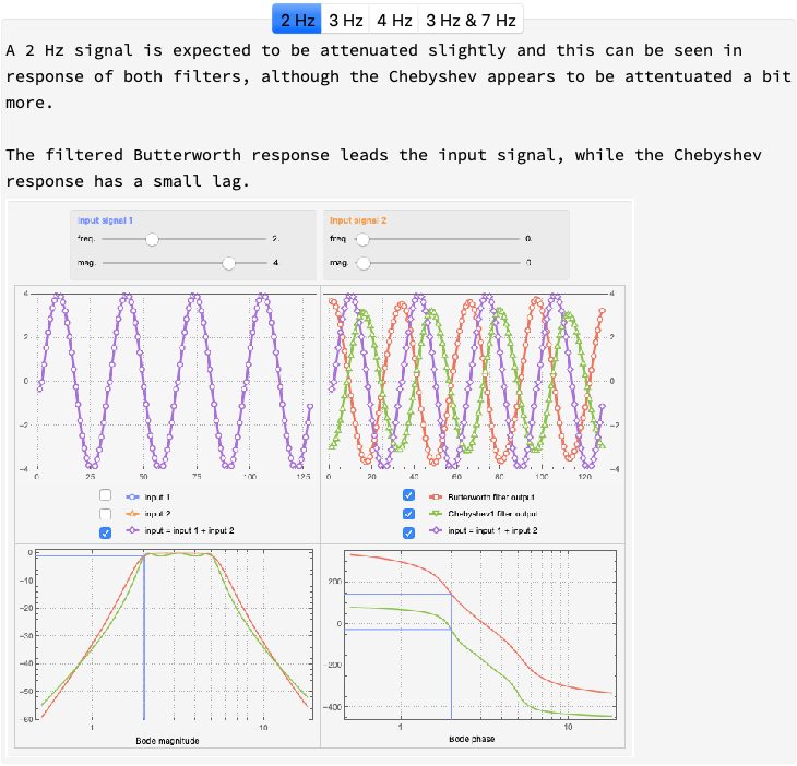
Finally, before disconnecting the Arduino, I remove the tasks and close the connection to the device.
TaskRemove /@ {taskObj1, taskObj2};
DeviceClose[dev]
Initialize the utility functions
A function to compute the phase in degrees.
Clear[phase]
phase[w_, i_ ] /; AllTrue[Unevaluated[{cw1, cw2, cw3}], ValueQ] :=
 With[{arg = Arg[Switch[i, 1, brw, _, cbs][w I][[1, 1]]]/Degree},
  Which[
   i == 1 && w < cw1, arg + 360,
   i == 1 && w > cw2, arg - 360,
   i == 2 && w > cw3, arg - 360,
   True, arg
   ]
  ]
phase[w_, i_ ] := (
  {cw1, cw2} = getCrossOvers[brw];
  {cw3} = getCrossOvers[cbs];
  phase[w, i]
  )
A function to compute the frequencies at which the phase crosses the negative real axis (180° phase).
Clear[getCrossOvers]
getCrossOvers[tfm_] := Block[{re, im, w},
  {re, im} = Chop[ComplexExpand[ReIm[tfm[I w][[1, 1]]]]];
  w /. NSolve[re < 0 && im == 0 && w > 0, w]
  ]
The functions to generate the lines showing the magnitude and phase of the filters at a specified frequency.
Clear[mLine, mLine1, pLine, pLine1]
mLine[w_ /; 0.5 <= w <= 18, c_] :=
 Join[{c},
  Table[mLine1[w, 20 Log10[Abs[tf[w I][[1, 1]]]]], {tf, {cbs, brw}}]]
mLine[___] := {}
mLine1[w_, mag_] :=
 Line[{{Log10[w], -60}, {Log10[w], mag}, {Log10[0.4], mag}}]
pLine[w_ /; 0.5 <= w <= 18, c_] :=
 Join[{c}, Table[pLine1[w, phase[w, i]], {i, 2}]]
pLine[___] := {}
pLine1[w_, arg_] :=
 Line[{{Log10[w], -460}, {Log10[w], arg}, {Log10[0.4], arg}}]
A function, along with supporting ones, to generate the input signals.
signals[w1_, g1_, w2_, g2_] := (signal1[w1, g1]; signal2[w2, g2];
  signalLengths; i1 = i2 = 1;)

signal1[args__] := in1 = signalGenerator[args]
signal2[ args__] := in2 = signalGenerator[args]

signalGenerator[w_ /; w != 0., g_] :=
 With[{signal = Table[g Sin[w  t], {t, 0, 2.0 ? /w, sp}]},
  signal]
signalGenerator[w_, g_] := ConstantArray[g, {20}]
A function to determine the signal lengths.
signalLengths := ({len1, len2} = Length /@ {in1, in2};
  lenM = 2 Max[len1, len2];)
A function to drop stale values.
drop[ls_] := With[{len = Length[ls]}, Drop[ls, Max[len - 2 lenM, 0]]]
A function to parse the incoming data.
parseData[{sB0_, sig1__, dB0_, sig2__}] /; {sB0, dB0} == {sB, dB} :=
 ToExpression[FromCharacterCode /@ {{sig1}, {sig2}}]
parseData[___] := Nothing
Load the paclet.
Needs["MicrocontrollerKit`"]
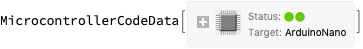
Assign the MicrocontrollerCodeData object to enable data acquisition without evaluating MicrocontrollerEmbedCode at each kernel startup (optional).
Set the plot styles.

And the legends.
With[{l1 =
List @@ FullForm[
ListLinePlot[RandomReal[{-1, 1}, {5, 20}],
PlotLegends -> Automatic, PlotStyle -> {cI1, cI2, cI, cB, cC},
PlotTheme -> {"Business"}]][[1, 2, 1]]},
lM = Flatten[Cases[l1, HoldPattern[ Rule][LegendMarkers, x_] :> x],
1];
l = l1[[1, All]];
]
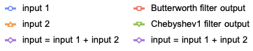
Grid[{{
lI = With[{i = {1, 2, 3}},
LineLegend[
l[[i]], {"input 1", "input 2", "input = input 1 + input 2"}[[
i]], LegendMarkers -> (lM[[i]])]]
,
lIO = With[{i = {4, 5, 3}},
LineLegend[
l[[i]], {"Butterworth filter output",
"Chebyshev1 filter output", "input = input 1 + input 2"},
LegendMarkers -> (lM[[i]])]]
}}]