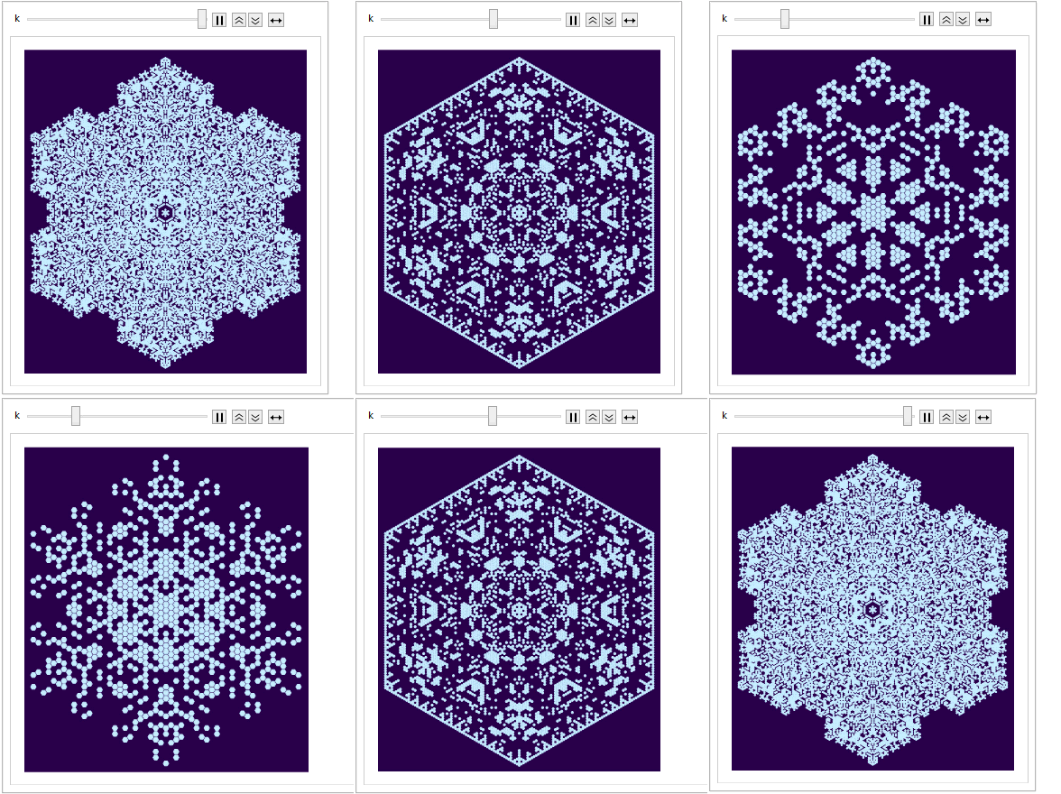
Some time ago one of my friends asked me whether it is possible to design a cellular automaton which can generate realistic snowflakes. I recall my crystallography and thermodynamics knowledge and came up a very simple yet impressive model.


The Regular Triangular Lattice

First of all, we are trying to simulate snowflake, which is a kind of hexagonal crystal. So it should be best to construct our CA on a regular hexagonal grid, i.e. regular triangular lattice.

We all know CellularAutomaton inherently works on rectangle lattices ("4-lattice" for short), so how can we deduce a triangular lattice ("3-lattice" for short) on it? Well, the differences between rect-lattice and triangular one is just a geometric transformation.

To demonstrate that, have a look at the following 4-lattice, with a blue square highlighting the range-1 Moore neighborhood:



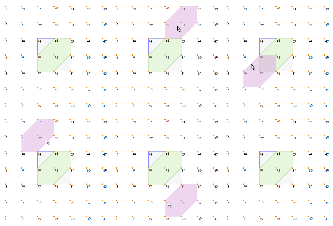
Clearly there is always a hexagon (the green area) in this kind of neighborhood.

So forming a regular 3-lattice is as straightforward as doing a simple affine transformation (basically a shearing and a scaling):



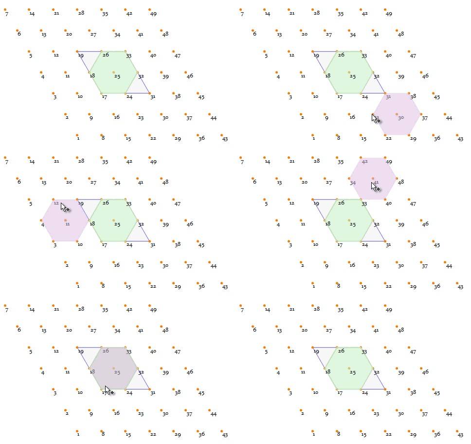
So to take advantage of all the power of CellularAutomaton, all we have to do, is to use a following special 6-neighborhood stencil on rectangle lattices, meanwhile our model can be discussed and constructed on regular triangular lattice convieniently:



And after the calculation, we can perform the affine transformation with following functions to get a nice hexagonal grid picture.




The Model

To construct the crystallization model, let's consider one of the 6-neighborhood stencil, where each cell represents a minimal crystal unit:



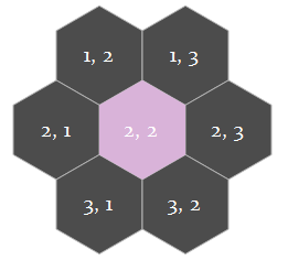
A simple model will need only 2 states: 0 for "It's empty", 1 for "There is a crystal unit". So by considering all (except the 000000 one, because we are generating ONE snowflake thus don't want a crystall randomly arises from void) 6-bit non-negative numbers, we can have a finite set of possible arrangements of the neighborhood:


However, from the viewpoint of physics, any two arrangements which can be transformed into each other with only rotation and reflection should be considered as the same arrangement in the sense of their physical effects on the central cell (i.e. cell2,2) are the same:



So we should gather stateSet with above equivalence class:


Which turned out to be 12 classes in total:



Now from the viewpoint of cellular automaton, we need to establish a set of rules on how should any 6-neighborhood arrangement, i.e. those 12 kinds of equivalence classes, determine the state of the central cell.

There are 4 kinds of possible transformations on cell2,2: 0 --> 1 is called frozen, 0 --> 0 is remaining empty, 1 --> 1 is remaining frozen, and 1 --> 0 is called melten. To make things more interesting and to explore more possibilities, we can introduce probability here, so certain arrangement will give certain probabilities corresponding to the 4 kinds of transformations. But notice that because of the unitarity of probability, we have Prob(frozen) + Prob(0->0) = 1 and Prob(melten) + Prob(1->1) = 1, so only 2 of the 4 probabilities are independent. In the following, we'll choose Prob(frozen) and Prob(melten), and denote them as pFrozen and pMelten.



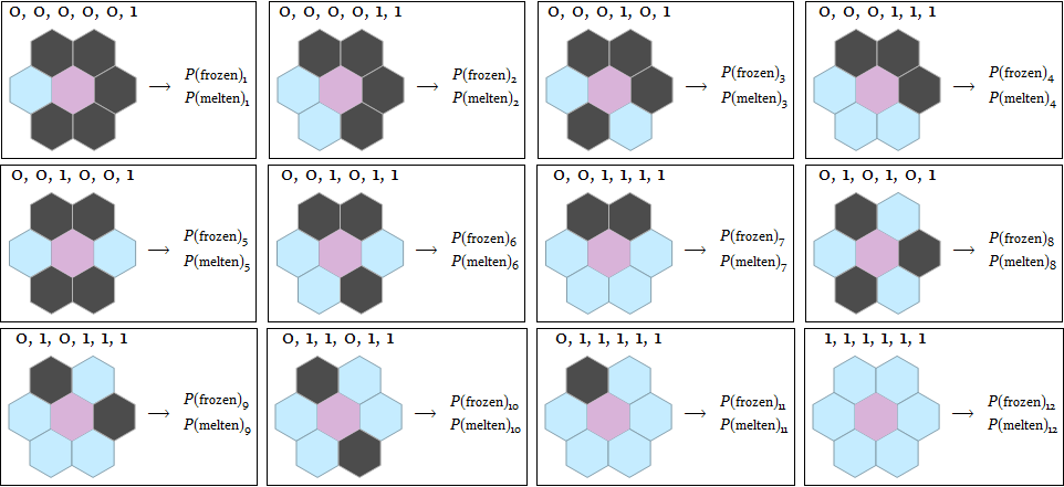
Back to physics / thermodynamics, those 24 probabilities, pFrozen and pMelten, can of corse be determined by serious physical models, or they can be chosen randomly just for fun. For example, an intuitive (and naive) idea would be to believe an empty cell nearby a sharp pointed end or with abundant moisture source will have a high pFrozen. (People who are interested in the serious physical models should not miss the Gravner-Griffeath Snowfakes model.)

Now we have the grid, the stencil, the neighborhood arrangement set and the transfer probabilities, we're offically ready to construct our cellular automaton rules.
Following the above discussion, the construction is straightforward. There are only two points which need to pay attention to. One is to keep in mind that the rule function is applied on the 3x3 stencil, so even cell1,1 and cell3,3 has nothing to do with our model, don't forget handling them. The second is to use a SeedRandom function to make sure same arrangement gives same result in same time step, otherwise the 6-fold rotational symmetry and 3 axes of reflection symmetry will both break!


(Note: re-compile the rule function ruleFunc will give a different set of seedStore thus a different growth path.)

Now everything is ready, let's grow a snowflake from the beginning!







Possible Improvements

We used a SeedRandom function in our CA rule function to force the 6-fold rotational symmetry and 3 axes of reflection symmetry, and performed the CA calculation on all cells. However, this so called D6 symmetry can (and should) be integrated into our model, which will saving 11/12 of the calculation. Also, the randomness of the growth path comes from seedStore, so to generate a new growth path, we have to re-compile the rule function. But with a improved model as described above, this constraint will no longer exist.




Open question 

Can we construct a well-organized structure (like the crystals) from a cellular automaton defined on an irregular grid? While I believe the answer is yes, the next question would be how?