I use the .flac audio file from
this link or you can directly download by clicking
here. I put the file under $HomeDirectory so I can import the file directly by its name, sample.flac.
{rate,duration}=Import["sample.flac",{{"SampleRate", "Duration"}}]
{8000,4.39938}
Load the data with "Data" option:
data = Import["sample.flac", {"Data", 1}];
timeSpot = Drop[Range[0., duration, duration/(rate*duration)], -1];
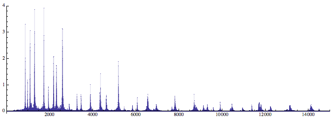
I can use the Fourier function to find the spectrum of the signal:
ListPlot[Abs@Fourier[data], PlotRange -> {{0, 15000}, All},
PlotStyle -> {PointSize -> Tiny}, Filling -> Axis,
AspectRatio -> 1/3]
The thickness/darkness of the trace in the spectorgram also shows which frequence is dominant. This graph is a partitioned spectrum:
Spectrogram[data]

Now I would like to add some low pass filters to attenuate some signal above 10Hz. In the simplest case, I use the following transfer function model:
sys = TransferFunctionModel[{{10/(s + 10)}}, s]
BodePlot[sys, AspectRatio -> 1/3,
PlotLabel -> {"Magnitude Plot", "Phase Plot"}]

I know this lowpass filter works from the bode plot. In the Magnitude plot, the "10" on the x-axis points at somewhat "-3" on the y-axis along the curve. At a given cut-off frequence, the component of a signal above this particular frequence should lose at least 50%. This is found by the definition of dB:
r^2 /. (NSolve[-20*Log10[r] == 3., r][[1]])
(*r^2 approx. 0.501 *)
where r is the magnitude and r^2 is the energy/signal strength.
I can also chain the two things together:

In the real application, I choose Wolfram System Modeler for quick prototype:
mmodel = "filter";
WSMModelData[mmodel]

Convert the count of points to the actual time spots:
f = Interpolation[Transpose[{timeSpot, data}]];
Input file in the System Modeler can be specified from within Mathematica:
model =
WSMSimulate[mmodel, {0., timeSpot[[-1]]},
WSMInputFunctions -> {"u" -> f}]
y2 = model[{"transferFunction.y"}][[1]]
y3 = model[{"transferFunction1.y"}][[1]]
The profile of the filtered signal:
Column[{
WSMPlot[model, {"transferFunction.y"},
PlotStyle -> Blue, PlotLabel -> "filtered once",
PlotRange -> Full],
WSMPlot[model, {"transferFunction1.y"},
PlotStyle -> Red, PlotLabel -> "filtered Twice", PlotRange -> Full]}
]

Use the default DFT functions to find the new spectrum:
ListPlot[ Abs[Fourier[y2 /@ timeSpot]][[1 ;; 1500]],
PlotLabel -> "Filtered Once",
PlotStyle -> {PointSize -> Small},
PlotRange -> All,
Filling -> Axis
]

Code for the filter.mo (annotation inclusive):
model filter
Modelica.Blocks.Continuous.TransferFunction transferFunction(b = {10}, a = {1,10});
Modelica.Blocks.Continuous.TransferFunction transferFunction1(b = {10}, a = {1,10});
Modelica.Blocks.Interfaces.RealInput u;
equation
connect(u,transferFunction.u);
connect(transferFunction.y,transferFunction1.u);
end filter;
Download the notebook from the link below
 Attachments:


