MODERATOR NOTE: GitHub repository containing SystemModeler files and the script to generate the data: https://github.com/DouwMarx/linear_regression_using_feedback_control
In this post, I show that the parameters of a linear model can be learnt by exploiting the time evolution of a dynamical system.
To demonstrate the goal of learning task, I start by showing an example of how the linear regression problem is usually solved. Then, I propose an alternative - An unusual parameter learning strategy, inspired by the gradient descent algorithm. For this learning approach, training data is treated as the inputs to a dynamical system. Optimal model parameters are then obtained from the steady-state properties of the time response of the dynamical system.
Finally, I discussing aspects of this approach I find interesting and speculate on possible extensions.
An example problem
We will use the dataset plotted below throughout this post. Our goal is to learn a model that can make generalisations from this data. A model answering the question: if we know $x$, what will $y$ be?
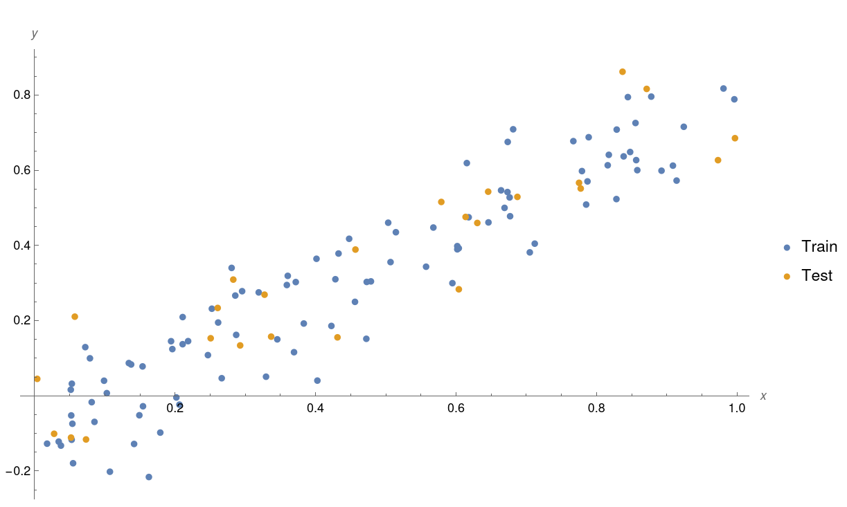
Looking at the data, it seems reasonable to fit a linear model of the form $y = w_1x + b_1$ with $w_1$ and $b_1$ the unknown parameters that we wish to learn from the data.
In fact, this is a very reasonable choice of model. The data you see here was generated using precisely this straight line equation with $w_1=0.9$, $b_1=-0.1$, and added Gaussian noise (standard deviation 0.1).
We use a synthetic dataset generated with known parameters so that we can later verify that the ground truth parameters are learnt.
Fitting a linear model to the data in an established way
Now that we have chosen a model, we can fit the model to our training data (Thereby learning the parameters $w_1$ and $b_1$). Here is an example of how it can be done in Mathematica:
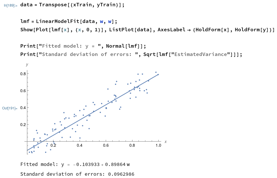
For linear models applied to small datasets, the parameter learning process typically reduces to a few elegant matrix multiplications (Ordinary Least Squares). In the process, the optimal parameters for the model is learnt from the data. We see that the recovered parameters are very close to the parameters that were used to generate the dataset ( $w_1=0.9$, $b_1=-0.1$).
A rather different approach to learning the model parameters
Now that I have shown the goal of this exercise, let's do the same thing, this time using a quite different approach. Would you believe that the dynamical system shown below serves the same purpose as the Mathematica code above?
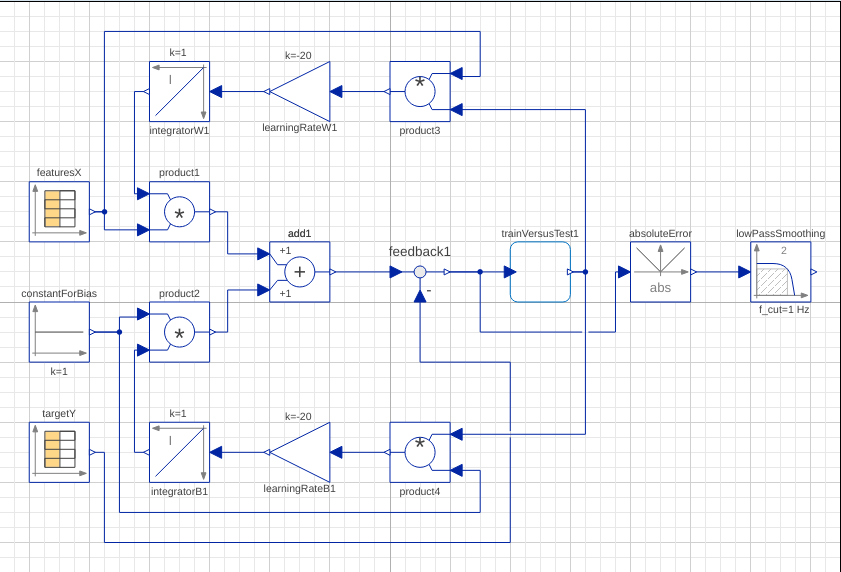
The picture shows a SystemModeler model of the dynamical system that we will be using to fit a linear model to data. If you don't know SystemModeler, you can think of it as a tool that can be used for studying dynamical systems. For example, to model this system, I connected summation, product, integration and table blocks. SystemModeler does the hard work of setting up the appropriate system of differential equations and solves for the time response.
How does it work?
Fitting a model to data can be viewed as an optimisation problem. We want to find the optimal parameters $w_1$ and $b_1$ that will enable us to make the best predictions of $y$ for a given $x$ in the future.
One possible approach to find good values for $w_1$ and $b_1$ would be to simply try thousands of combinations of $w_1$ and $b_1$ and choose the combination that fits the data the best. But there are more efficient ways to do this!
Inspiration from the gradient descent algorithm
A popular method for solving the optimisation problems encountered when fitting machine learning algorithms is the gradient decent algorithm (And its close relative, the stochastic gradient descent algorithm).
The gradient descent algorithm is powered by a metric that quantifies how well the model is fitting the data. This is called the loss function or objective function. A commonly used loss function is the square of the error between the data and the model prediction. High loss values indicate that the model is not fitting the data well. The true value of this loss function (and many other machine learning elements) lies in the fact that it is differentiable - We can calculate the gradient of the loss with respect to the model parameters. This gradient information is exploited by the gradient descent algorithm, and also in the method proposed in this post. Therefore, makes sense to elaborate a little further on the workings of the gradient descent algorithm.
How the gradient descent algorithm uses, Uhm... the gradient.
First, the loss for a starting set of parameters, for instance, w1=0 and b1=0 is calculated. This might lead to a terrible model fit and consequently, a very large loss. Now, instead of continuing to try other combinations of w1 and b1 at random, the values of w1 and b1 are updated in a direction that we know will lead to a decrease in the loss and consequently an improved fit of the model to the data. We know this direction from the derivative of the loss function.
$ L =\sum_{i=1}^{m} ( y_i - \hat{y_i})^2 $
Where $\hat{y_i}$ is the prediction of the model for a given set of parameters, $y_i$ is the $y$ value of the $i^{th}$ training sample and $m$ is the number of training samples.
Substituting $ \hat{y_i} = w_1 x_i + b_1$ we obtain
$ L =\sum_{i=1}^{m} ( y_i - (w_1 x_i + b_1))^2 $,
from which we can find the partial derivatives with respect to the model parameters $w_1$ and $b_1$.
$ \frac{dL}{dw_1} =\sum_{i=1}^{m} 2(y_i - (w_1 x_i + b_1)) \times -x_i $
$ \frac{dL}{db_1} =\sum_{i=1}^{m} 2(y_i - (w_1 x_i + b_1)) \times -1 $
To decrease the loss and improve the fit, we just have to shift the parameters in the opposite direction of the gradient of the loss, since this will lead to a decrease in the loss.
How this idea is used to let a dynamical system learn.
We take inspiration from the gradient descent technique by updating the model parameters in the direction that would lead to a decrease in the total loss and therefore improve the fit of the model to the data.
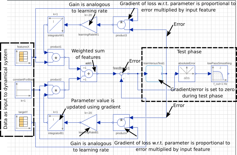
Have a look at the furiously annotated diagram below. The main idea is that a quantity, proportional to the input features multiplied by the error (the gradient for a squared error loss function) is fed back to an integrator to be "remembered".
A more detailed explanation of the function of each of the components follows.
What does each of the components do?
- The data table block (featuresX, targetY): This block presents the x and y values of a given training sample every $0.01$ seconds and keeps it constant ("step input") for that duration.
- The bias $b_1$ in the model is represented as $1 \times b_1$. This is often done in machine learning when working with a design matrix.
- The data for the table blocks is multiplied with weights ( $w_1$ and $b_1$) and summed. In the process, the prediction $\hat{y} = w_1 x_1 + b_1$ is computed for a given time step (A sample in the training set every $0.01$ seconds)
- Next, the error in the prediction due to the current best model parameters is computed. This is done by computing the difference between the target variable $y$ and the prediction $\hat{y}$
- Now, the error, multiplied with the input feature ( $x_1$ or $1$) is multiplied with a gain and fed into an integration block. This feedback quantity is proportional to the gradient of the loss function for a given set of model parameters. The gain block determines how aggressively the model parameters should be updated in the opposite direction of the gradient and in analogous to the learning rate in machine learning.
- The value of the integration blocks represents the current best set of weights ( $w_1$ or $b_1$) for the model.
- The value of the integrators are updated through time until it converges to the optimal set of parameters.
- The testTrain block is not important for understanding how the system learns. It is simply used to switch between the training (first $7$ seconds) and testing phases (last $2$ seconds) of the simulation. More on this shortly.
- The absolute value and the low-pass filter is only used during model evaluation.
What is happening during the simulation?
The training data is presented to the dynamical system several times during the training (Analogous to training epochs in machine learning). After about $7$ seconds, the values of the weights of the model ( $w_1$ and $b_1$) converge to a steady-state value. To stop the training, the feedback of the error is switched off and as a result, the weights remain constant in their trained and close-to-optimal state. In the spirit of machine learning with dynamical systems, the evaluation phase is also done within the same framework.
The results of the learning process
The figure below shows values that the integration components (the weights $w_1$ and $b_1$) take with time. Their values are initialized as zero. As samples are fed through the system with time, the parameter $w_1$ approaches $0.9$ and the parameter $b_1$ approaches $-0.1$. This result is consistent with the parameters that were initially used to generate the data set. The dynamical system has successfully learnt the near-optimal parameters for the linear model.
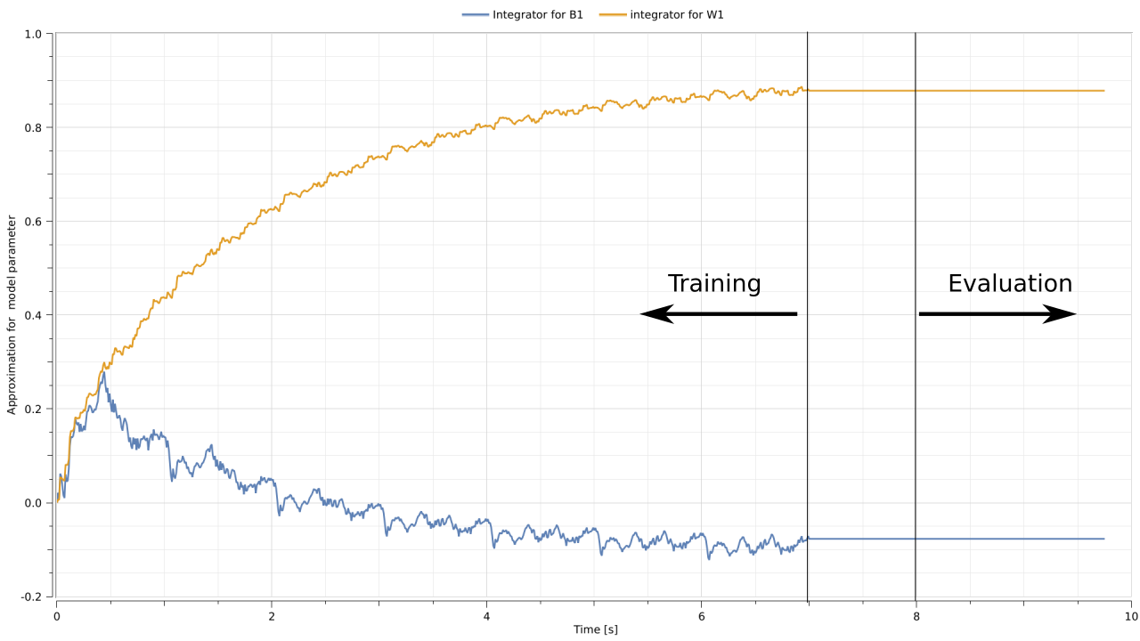
After $7$ seconds (and several epochs) of training, the gradient is no longer fed back to the integrators. A pause of $1$ second follows whereafter the evaluation phase starts.
From training to testing
It is good practice to evaluate how well a model is generalizing by evaluating its performance on new data that the model was not trained on. The new data is called the test set. In the spirit of machine learning with dynamical systems, we will perform the evaluation on the test set using the same dynamical system framework. During evaluation, the model weights remain constant as the samples are presented to the system and the prediction error is calculated with the same components used to compute the error during training.
The figure below shows the evolution of absolute error during the simulation. During training, the error decreases as the optimal parameters are learnt. During testing, the error serves as an indication of how well the learnt model is generalizing to new data.
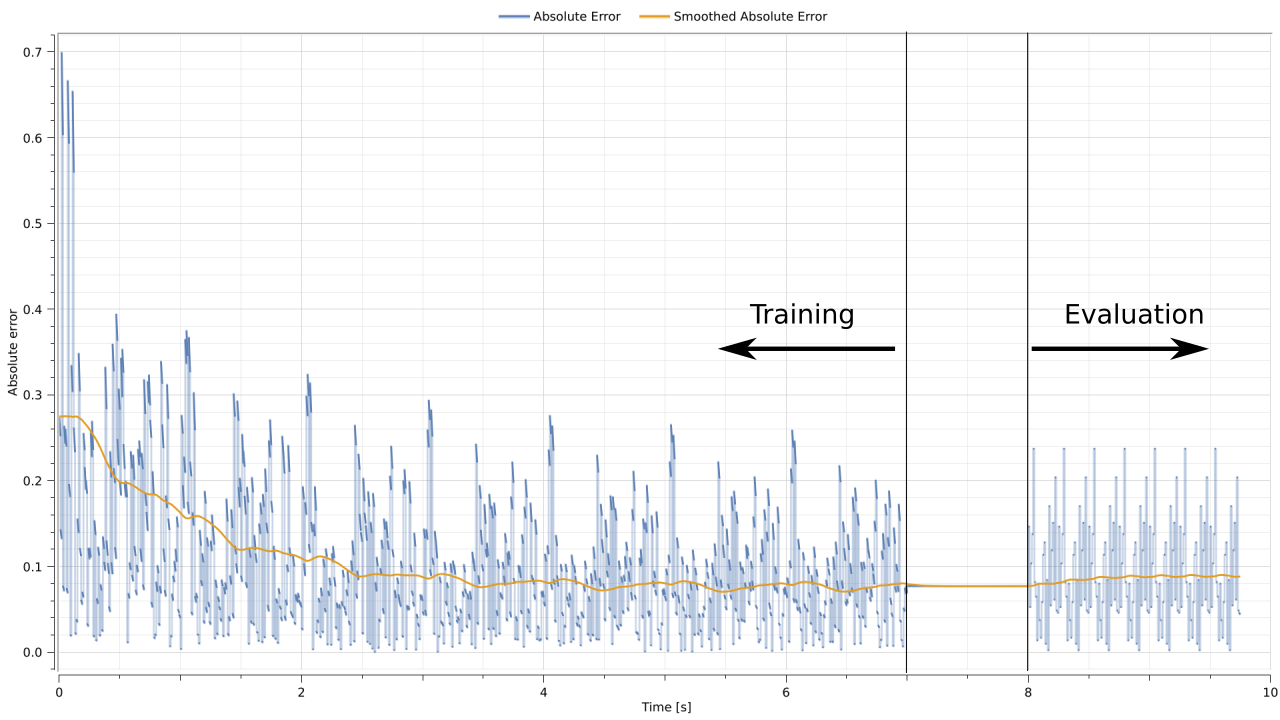
This error signal is also smoothed to represent the average error on the test set. The smoothed signal remains constant at roughly an absolute error value of $0.1$. This value is consistent with the standard deviation of the Gaussian noise that was used when generating the data.
Thats it!
A dynamical system can be used to learn the parameters of a linear model from data.
Epilogue: Some things I find interesting
This final section includes some thoughts related to this idea, some of them bordering on speculation.
- The fact that this idea employs basic "mathematical operations" that are common in dynamical systems implies that optimisation problems in machine learning could be solved using physical machines other than your computer CPU or GPU. In principle, an electric circuit, a network of water tanks or a spring-mass system can be used to solve optimisation problems.
- This idea could be extended to incorporate multiple features and non-linear activation functions to train neural networks through backpropagation.
- The training of models using dynamic systems could be efficient. Electrical dynamical systems could work through training samples at the order of GHz with "computations" for a given sample being performed in parallel. The bottleneck in the training speed might be at presenting the samples (digital to analogue conversion) and not in the actual number crunching that we associate with classical computing.
- It could be possible to used more elaborate loss functions and employ a differentiator to directly compute the signal that should be fed back to the integrator without requiring knowledge of the analytical gradient of the loss function.
- Other ideas from convex optimisation such as momentum and AdaGrad can be incorporated into the dynamical system. Gradients can be smoothed with a low pass filter as a way of adding momentum, and the learning rate (gain) can be adjusted as a function of the gradient.
- Smoothing of the weights could be interesting. The sudden termination of training in the example in this post means that the final set of learnt weights could be sensitive to the last sample that was shown to the system. Adjustments to the learning rate could address this issue, but the values of the weights could also be low-pas filtered for less noisy weights.
Fine print
- SystemModeler files and the script to generate the data are available here
- Any comments, corrections or recommendations will be appreciated.
- It can make sense to shuffle the data that are presented with each epoch. Patterns are visible in the absolute error with time as the samples in the training data is presented in the same order for each epoch.
- It would be more responsible to standardise that data before training.
- The number of epochs, learning rate and initial values for the weights were chosen to make the explanation as clear as possible.


