How can we increase accessibility of physics and math via the Wolfram Language? In this post, I would like to find out how an introductory usage guide can allow these formulas to be implemented with ease.
quantities = {"Mass", "Distance", "Time"};
targetQuantity = "Work";
workCombinations =
  DimensionalCombinations[quantities, targetQuantity,
   IncludeQuantities -> "PhysicalConstants"];
workCombinations

In Mathematica, we can define some really fundamental physical quantities like mass, distance, and time. How do we express these desired physical quantities in the form of work? The dimensional combinations is considering all these things like the speed of light, the gravitational constant, and the combinations of dimensions that represent work..these are the coefficients & exponents that make it possible to produce different valid combinations. Look at all those physical constants that we have available!
mass = Quantity[75, "Kilograms"];
height = Quantity[28, "Meters"];
workAgainstGravity =
 FormulaData[{"Work", "Gravity"}, <|
   QuantityVariable["m", "Mass"] -> mass,
   QuantityVariable["h", "Height"] -> height|>]
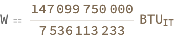
You can actually see the structure it's different as you get closer to the center of gravity..you know about those black holes where time is always being computed from the previous state, this giant graph and the pieces of the graph, are being rewritten. The progress of time is the progressive rewriting of the universe. As you get closer to the center of a black hole, you might get a response! You don't realize anything, there's no thinking going on. Frozen in time, the computed work against gravity is represented or compared in terms of the InternationalTableBritishThermalUnits that we call BTUs. It's pretty clear that there's a huge amount of work being done for this single 75-kilogram object that moves vertically 28 meters. In a time-like similarity, there is no extent to space. Oh certainly! You can model the work done against gravity for an object of specified mass that moves vertically over a specified distance like that.
mass = Quantity[Around[75, 0.1], "Kilograms"];
height = Quantity[Around[28, 0.1], "Meters"];
workAgainstGravityUncertain =
 FormulaData[{"Work", "Gravity"}, <|
   QuantityVariable["m", "Mass"] -> mass,
   QuantityVariable["h", "Height"] -> height|>]
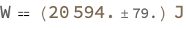
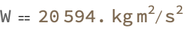
It really depends on what kind of scenario you're looking for when the universe expands forever but the rate increases, and eventually everything gets so far apart, that eventually nothing interesting can happen anymore. The result is the work done against gravity, represented as 20593.965 Joules. This means that yes the computed work is approximately 20593.965 Joules but due to uncertainties in the input values which are mass and height, the value might be off by as much as maybe 78.508 Joules. The associated uncertainty is derived from the uncertainty inherent within the mass and height of the specified object. We're existing in the transient before the real outcome of the universe is known.
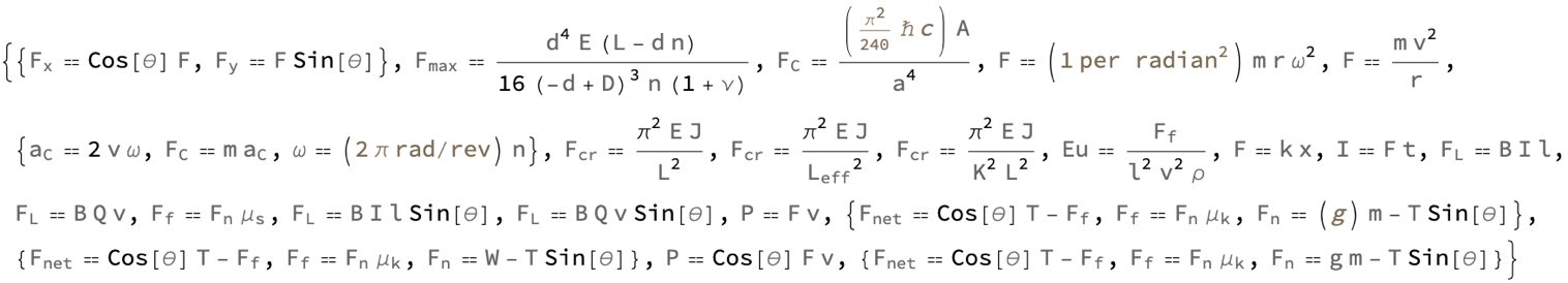
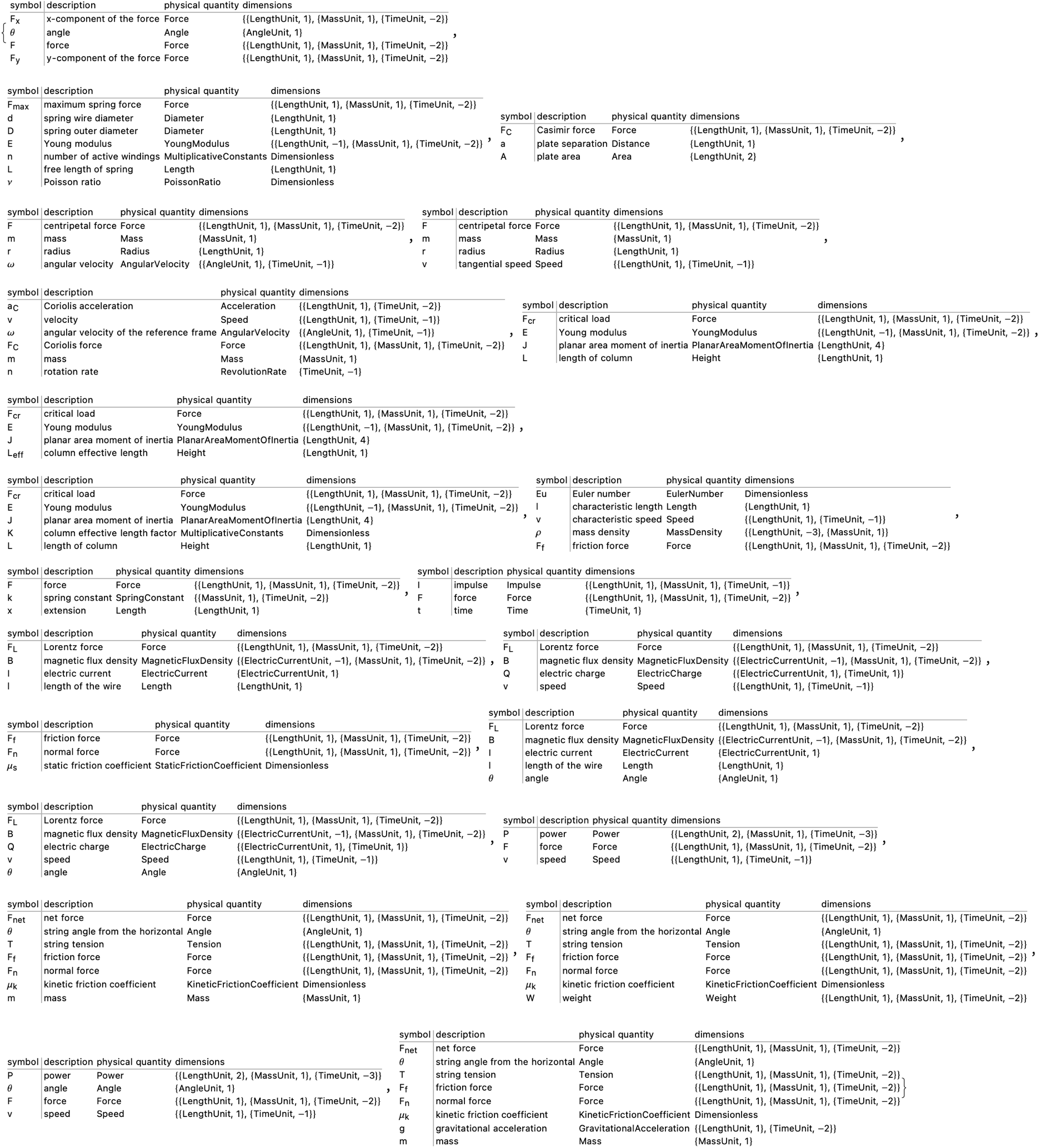
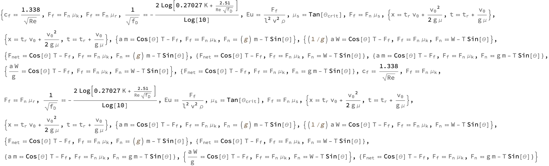
frictionFormulas = FormulaLookup["Friction"];
frictionComparison =
 Table[FormulaData[formula, "QuantityVariableTable"], {formula,
   frictionFormulas}]
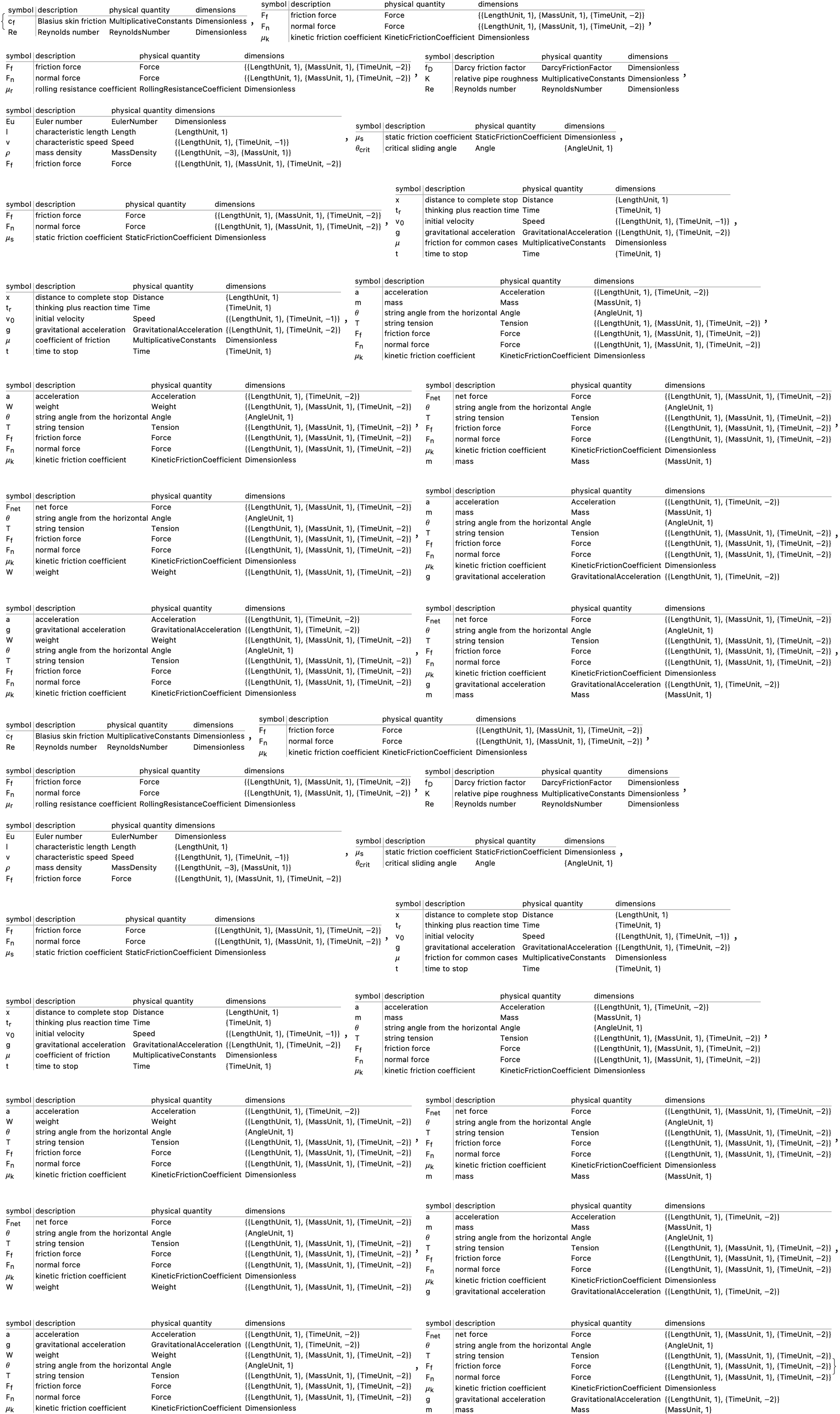
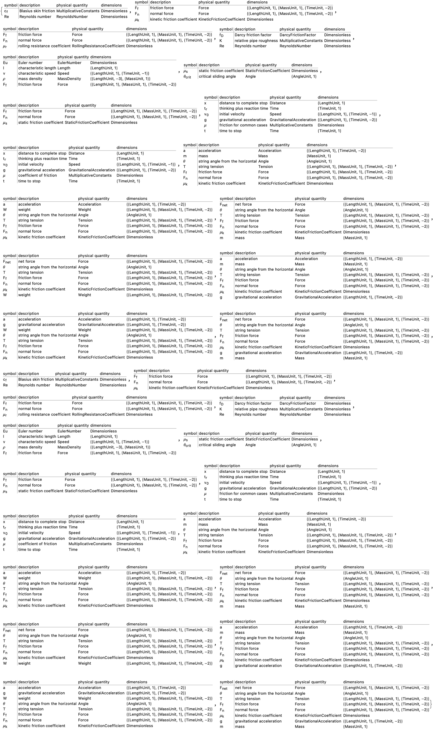
If you actually care about the formulas related to friction that are available in the database of formulas that are built-in to Mathematica, and there are user-provided functions..you can fetch this assortment, it's just another formula in the quantity-variable table that we use as a way to retrieve a table of quantity-variables associated with the friction formula, which allows us to gain a clearer understanding of what variables and their dimensions or units, how are they involved in each friction-related formula, and how they correspond to the kinetic friction coefficient, and the rolling resistance coefficient, and the things that correspond to different Euler numbers; insert characteristic variable here.
GetFormulasRelatedTo[quantity_String] :=
 Table[FormulaData[formula], {formula, FormulaLookup[quantity]}]
GetFormulasRelatedTo["Energy"]

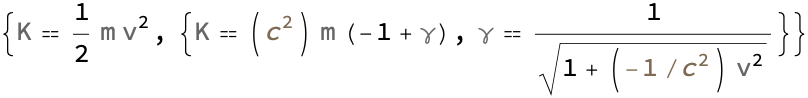
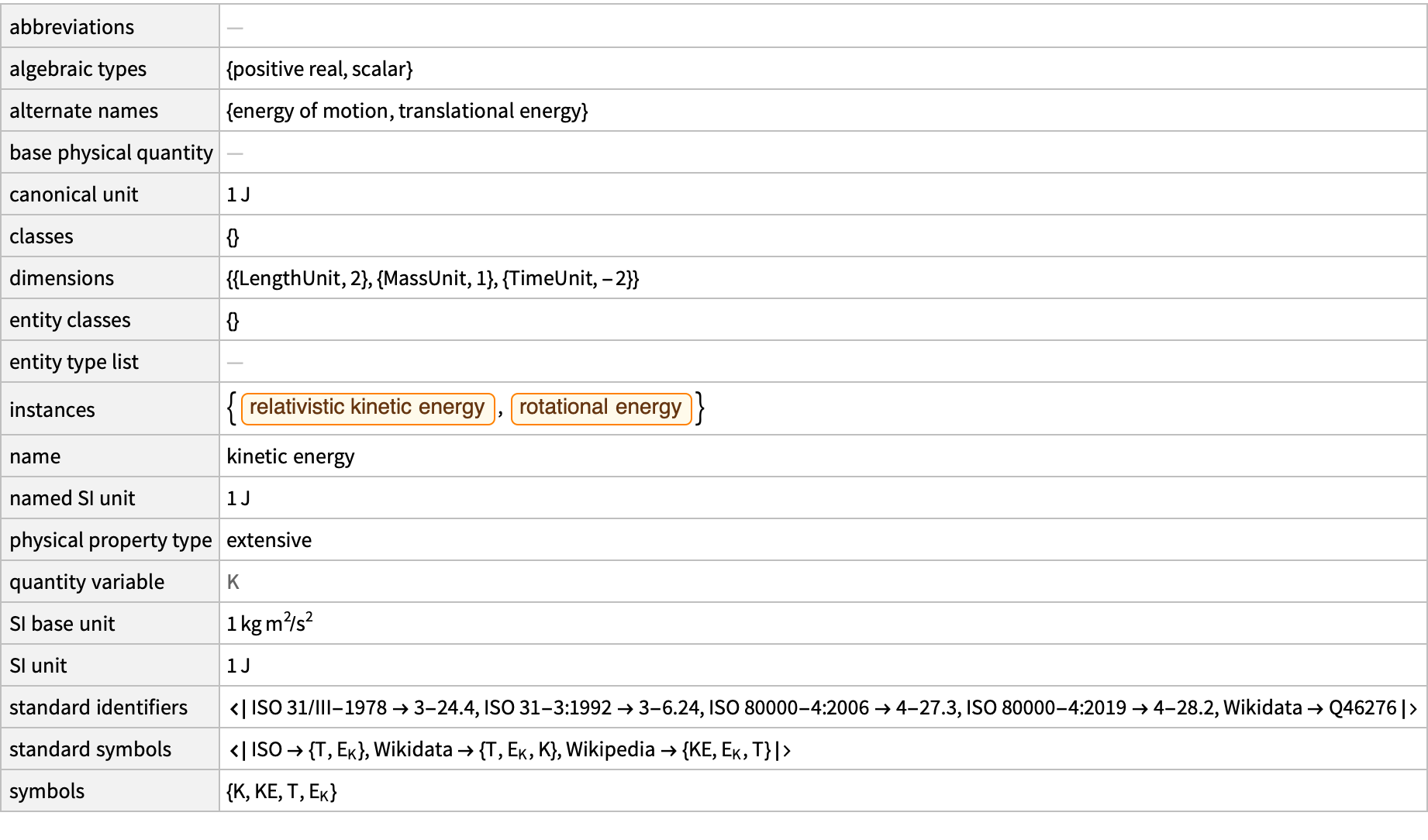
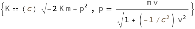
The formulas that are associated with the physical quantity known as energy which is what comes out, when you take a string input that represents the physical quantity energy, and retrieve all the energy-associated formulas, these are the classical expressions for kinetic energy, specifically energy in the context of relativity. But is that true? We can't generalize the energy itself, however we can express the energy K in terms of the mass m and the gamma factor γ. The particle is just left hanging on its own and that emerges as a piece of radiation coming out from the black hole, which is in turn given as a function of speed v and the speed of light.
GetFormulaProperties["Energy"]

If you're falling into a black hole and a certain amount of time elapses you seem like you're slowing down and slowing down, and slowing down you know, it will be as if that clock was ticking slower and slower at the glowing threshold of the event horizon. The keys are the formula identifiers like KineticEnergy and KineticEnergyRelativistic which is why the values that are the results of the function FormulaDataPropertyAssociation that are applied to the formula identifiers. In Russian physics, black holes were called frozen stars; it looks sort of like everything freezes. That's what happens, so to an observer, it freezes at that level; while this function is the classical formula for kinetic energy, in a relativistic context, we can gain an embedded understanding of the branching properties and attributes, of the formula specified.
VisualizeUnitRelations[quantity_Entity] :=
 SimpleGraph[
  RelationGraph[#1["SIUnit"] == #2["SIUnit"] &,
   RandomSample[
    ResourceFunction["PhysicalQuantityLookup"][
     quantity["SIBaseUnit"]], 10]], VertexLabels -> Automatic]
VisualizeUnitRelations[Entity["PhysicalQuantity", "Speed"]]
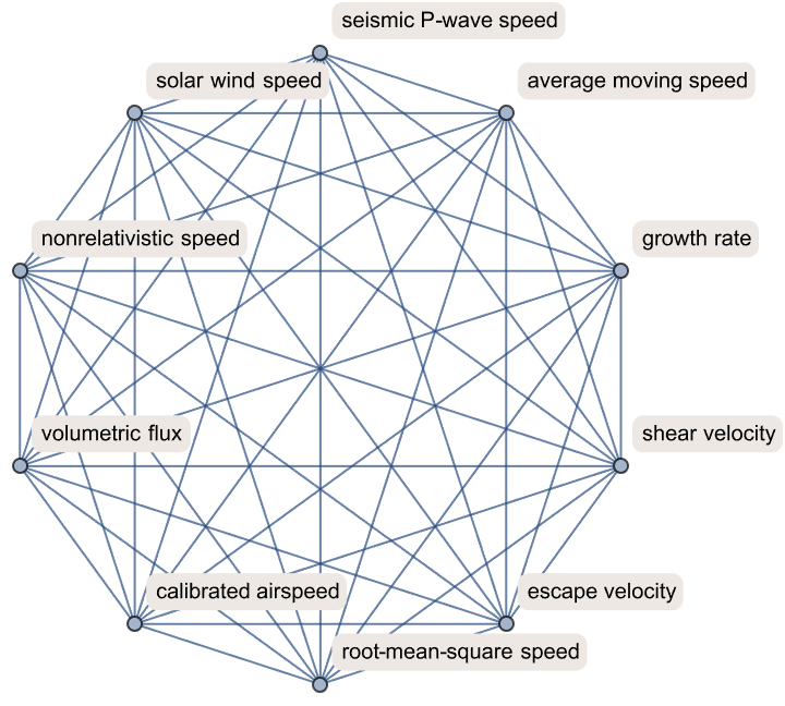
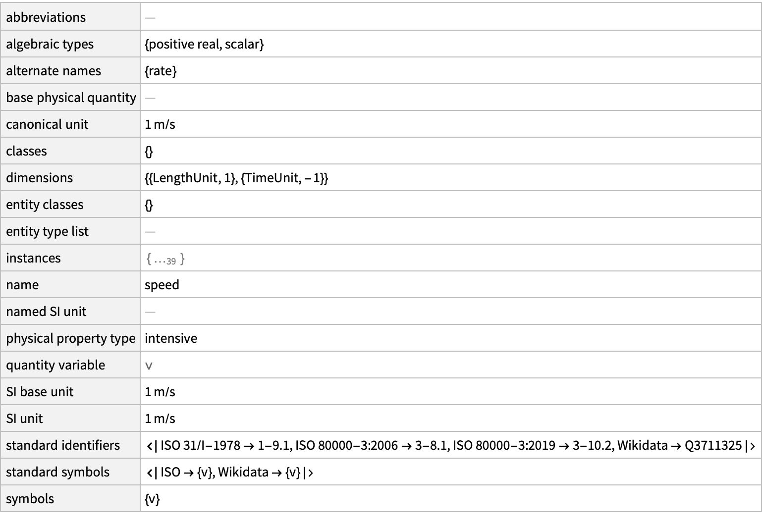
The International Standard of a specified physical quantity which from which can be derived relationships between different SI units, it's possible for certain SI units of the Entities of type PhysicalQuantity to be defined, right? We had that all along, since epochs ago where the same mathematics was used for three completely different purposes; we can define a predicate function that checks if two entities have the same SI unit, and then take a random sample of 10 related physical quantities via the PhysicalQuantityLookup, which, fetches related physical quantities that share the same SI base unit, as the provided quantity. The vertices can be labeled via wrapping the resulting graph with SimpleGraph and it didn't work, that is all. The previously defined function, with the physical quantity speed, confiscates all different SI units related to speed and provides a visual representation that has always been a part of our vocabulary: there's kind of this theory about how particles work in terms of these wave equations..in our models of physics the electron is not infinitely small but it's pretty small compared to the kind of things we can measure in particle accelerators today.
Plot3D[\[Mu]k*NormalForce, {\[Mu]k, 0, 1}, {NormalForce, 0, 10},
 AxesLabel -> {"\[Mu]k", "Normal force", "Friction force"},
 PlotRange -> All,
 PlotLabel -> "Friction force for your coefficients & normal force"]
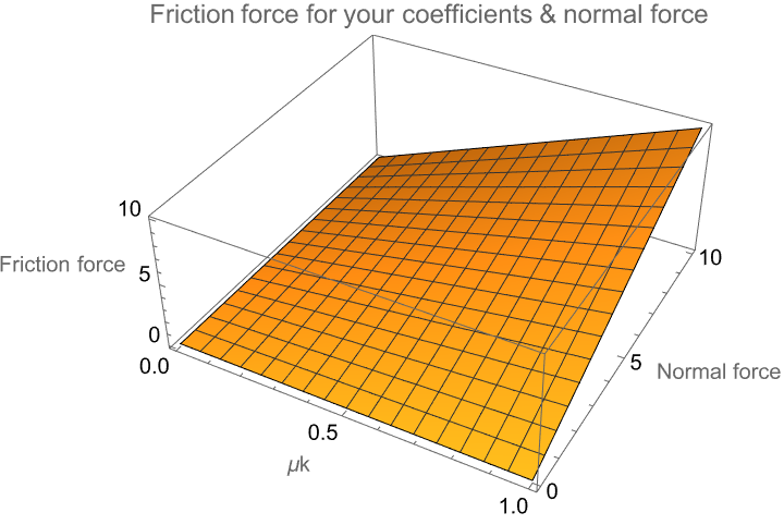
When variables leak outside of their scope, we can generate a 3D plot to visualize the relationship between the frictional force, the coefficient of kinetic friction μk, and the normal force. That is how we find the frictional force that is the product of the coefficient of kinetic friction and the normal force. That's why moon rock is worth it's worth because the moon soil, consists of these sand-like granules, and varying the coefficient of kinetic friction and the normal force affects the frictional force. That's the surface that has a sequel, that slopes upward as either μk or the NormalForce increases, given their direct relationship with the frictional force. In other words, μk ranges from 0 to 1, and the NormalForce ranges from 0 to 10.
WorkUnderVariableForce[forceFunction_, {x_, xStart_, xEnd_}] :=
 Module[{work, plot},
  work = NIntegrate[forceFunction, {x, xStart, xEnd}];
  plot =
   Plot[forceFunction, {x, xStart, xEnd}, Filling -> Axis,
    FillingStyle -> LightGray,
    PlotLabel -> "Area represents work done"];
  {work, plot}]

WorkUnderVariableForce[2*x + 3, {x, 0, 10}]
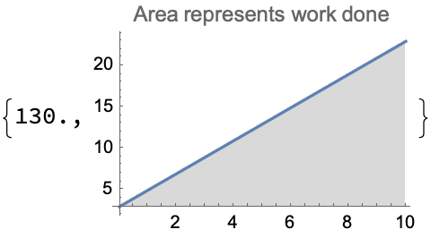
When you apply the variable force function over a specified displacement, when you apply it to compute and visualize the work done via the WorkUnderVariableForce function that takes in two arguments where x is the variable of integration and xStart and xEnd are the limits of integration, or the range over which the displacement occurs, the work done by the variable force shows up and saves us the trouble and allows us to escape the area that represents the work done under the curve, and then the numerical integration provides us with the visual representation of the variable force as a function of x.
Table[FormulaData[formula], {formula, FormulaLookup["Power"]}]
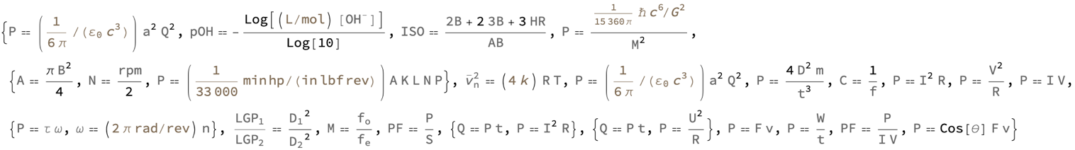
It's yours, the FormulaLookup that gets a list of formula IDs that are related to Energy, and the FormulaData that is applied to each ID to fetch the actual formula; there are various outer space treaties for who exactly would get upset if you start writing your ad in space. So to speak! The results are presented as a list of equations following our queries of the formulas related to Energy and Power for which the formulas for Energy include the formula for kinetic energy and a formula related to relativistic energy. The variety of formulas like electric power, mechanical power, the wrinkle in time of the solid tides that they actually produce heating in the moon and that heating produces volcanoes and all kinds of stuff..relationships involving torque and angular velocity, and more expansion. And then the Wolfram Language database comes in and messes up the formulas so we can quickly retrieve the formulas related to Power.
Plot3D[30 x y, {x, 0, 10}, {y, 0, 10},
 AxesLabel -> {"Force (N)", "Distance (m)", "Work (J)"}]
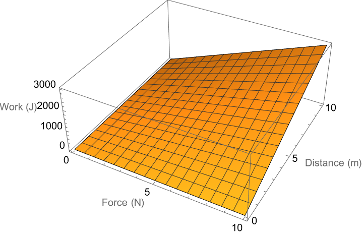
This time, you're the one breaking down a 3D surface and you're going to do it using the Plot3D function that the Wolfram Language provides. What is the surface? On this surface, there are layers of moon rock that have not seen the sun for billions of years but over the course of decades they get bleached back into color. The z-value that is the height at any point on the xy-plane, what is it? Well, it's given by the product 30xy. The variable x and the variable y are our stalwarts of the surface that allows the product of force in Newtons and distance in meters to be scaled by a factor of 30. I kind of block it out which is terrible, what the visual demonstration is these days of the relationship Work = 30 * Force * Distance over the specified ranges of force and distance.
UnitConvert[Quantity[1, "Joules"], "Calories"]
UnitConvert[Quantity[1, "Joules"], "Electronvolts"]

It's the conversion from Joules to Calories, how charming. That's a strange fish, I don't know what caffeine does to fish. What I do know is that cats do badly with Tylenol because the kidneys of humans kind of filter that out of our bloodstream but that doesn't work with cats...normally, Mathematica will provide you with the numerical values that make these conversions possible. You want to have a kilo, you want to have a redo, you want to have the 1 Joule that is approximately equal to 2.39006 * 10^-4 Calories which is the nutritional definition of a Calorie, so when you actually do it it should only take two minutes of your time: it's the kilocalorie in thermodynamic terms! What is 1 Joule? 1 Joule, is equivalent to approximately 6.242 * 10^18 electronvolts which is transcendentally impressive. It's the obituary of the numerical values which are derived to convert a quantity measured in Joules into other units. The first conversion is from Joules to Calories. The second conversion is from Joules to Electronvolts. Which one is it?
Entity["PhysicalQuantity", "Energy"]["Dataset"]

Table[FormulaData[formula, "QuantityVariableTable"], {formula,
  FormulaLookup["Energy"]}]

The two main formulas associated with energy are a very weird phenomenon. The involvement of relativistic energy wherein K is the energy, m is the mass, γ is the Lorentz factor - Gamma is the relativistic factor, v is the speed - look up how the speed of light is implicitly involved in the formula! You don't want to - could there be a golden asteroid? The way that we query and represent formulas related to the physical quantity of energy is the detailed representation that the Table constructs via the FormulaData[formula] that exists for each of these formulas: the structured, tabular representation of data in Mathematica is back! How did it come about?
DimensionalCombinations[{"Mass", "Length", "Time"}, "Energy"]

What we can do is indicate the dimension of energy consistently with the definition of energy in the SI unit system in which energy in joules is equivalent to meter^2 * kilogram / second^2. What this means is that the three-dimensional parametric plot can be scheduled, it can be plotted:
ParametricPlot3D[{x, Sin[x - t], t}, {x, 0, 10}, {t, 0, 10},
 PlotRange -> All, AxesLabel -> {"Space", "Amplitude", "Time"}]
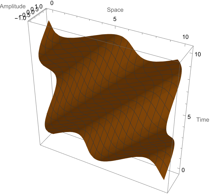
The Space axis corresponds to the value of x and the Amplitude axis corresponds to the Sin[x - t], which is a way of representing a wave of shifts based on the value of t, t which corresponds to the Time axis. In that sense we can reschedule the entire range of the function such that it's shown in the plot. I think what's true is that there is a certain level of looking for obvious things where you know the diagnosis and you know what you're looking for that's AI-accessible; what's the thing trying to figure out; do you have diagnosis X? I think that has more potential than will this thing turn out to grow more or do this thing or what-ever that's more well defined. Such as the dimensional combinations for energy, wherein the three-dimensional waveform in space and time can be, and I don't know if you're reading this, but it is possible to return the possible combinations of dimensions that result in the desired dimension.
workByGravity =
 FormulaData[{"Work", "Gravity"}, <|
   QuantityVariable["m", "Mass"] -> Quantity[75., "Kilograms"],
   QuantityVariable["h", "Height"] -> Quantity[28., "Meters"]|>,
  UnitSystem -> "SIBase"]
Those different use cases can have different consequences there; to compute formulae related to specific physical phenomena such as work and friction, the specific Moore's law like curve particularly involving work and friction. How many fall-throughs occur and how can we analyze them and make them work better? The Wolfram Alpha, we saw a kind of exponential improvement up to a high success rate for many different things; we can retrieve the formula for work done by gravity, and then input specific values for mass (75 kg) and height (28 meters) wherein we can calculate the work. UnitSystem -> "SIBase" is what specifies that the result should be given in SI units.
frictionFormulas =
 Table[FormulaData[formula], {formula, FormulaLookup["Friction"]}]
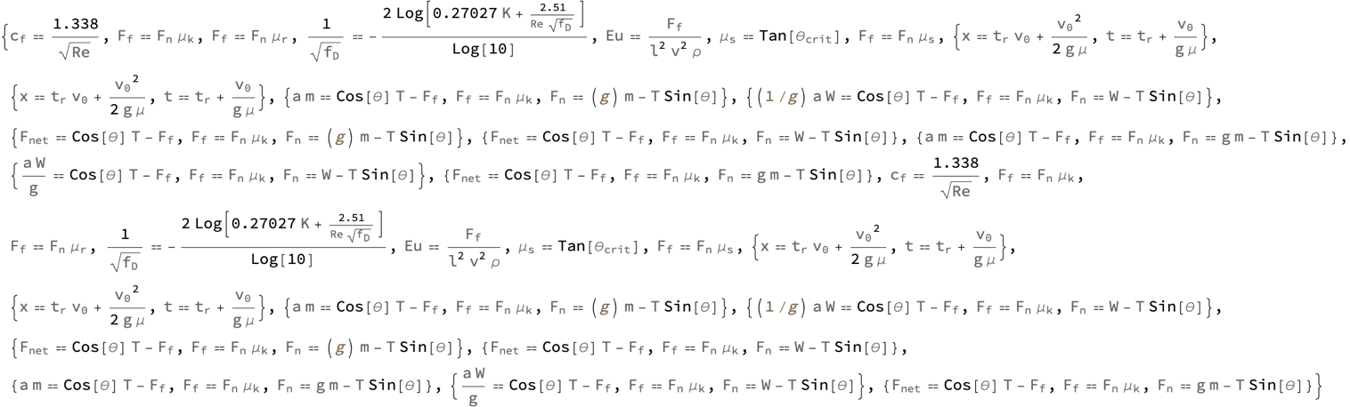
When you display the formulae involving friction it's a little soft, the frictional forces, the coefficients and the other related quantities, and there's a lot to unpack there because the static and kinetic friction, Reynolds number, and Darcy friction factor..all of these things we don't have to wait for; we can simply break down this table and then take a look at the coefficient of friction due to the Reynolds number, or the force due to kinetic friction as the product of the normal force and the kinetic friction coefficient. We can grab the force of friction and how it relates to the rolling resistance coefficient. The static friction coefficient isn't so static, it typically is given based on the critical angle of friction which keeps vacillating up and down the incline which just might be because the scenarios involving inclined planes, fluids, and specific coefficients, they need to generate and compute these formulae values based on inputs that they haven't done naturally.
forceFormulas =
 Table[FormulaData[formula], {formula, FormulaLookup["Force"]}]
replaceVariablesInDimensionalCombination[combination_,
  replacements_] := UnitSimplify[combination /. replacements]

workWithSpecificValues =
 replaceVariablesInDimensionalCombination[
  DimensionalCombinations[{"Mass", "Distance"}, "Work",
   IncludeQuantities -> {Quantity[1,
      "StandardAccelerationOfGravity"]}], <|
   QuantityVariable["Distance"] -> Quantity[10.3, "Meters"],
   QuantityVariable["Mass"] -> Quantity[46., "Kilograms"]|>]
The question is are those words that we care about or not? The same thing happens with music. You can put together many sequences of notes and many people would just say that sequence of notes sounds terrible..that resonance with us is related to things that we are already familiar with; those are the language, the intrinsic characteristics that we as humans have that make sense to us; the computational characteristics of the formula names related to force for which the actual formula for each of those names, and the way that we can replace the variables in a given dimensional combination with the ReplaceAll function /., that is generated with specific values so that we can then simplify the unit, if it isn't your first time, if it isn't your list of formulas related to force right before we define this custom function that replaces variables in dimensional combinations which faithfully reminds us of the specific work value by considering the gravitational force, acting on a 46-kilogram mass at a distance of 10.3 meters, we might say that we introduce new words into the language and we equivocate between InternationalTableBritishThermalUnits and the "constant for standard gravitational acceleration".
workWithDifferentAngles =
 Table[FormulaData[{"Work", "Standard"}, <|
    QuantityVariable["d", "Distance"] -> Quantity[50, "Meters"],
    QuantityVariable["F", "Force"] ->
     Quantity[30, "Newtons"] Cos[\[Theta]]|>], {\[Theta], 0, Pi/2,
   Pi/10}]
Table[FormulaData[formula], {formula, FormulaLookup["Velocity"]}]
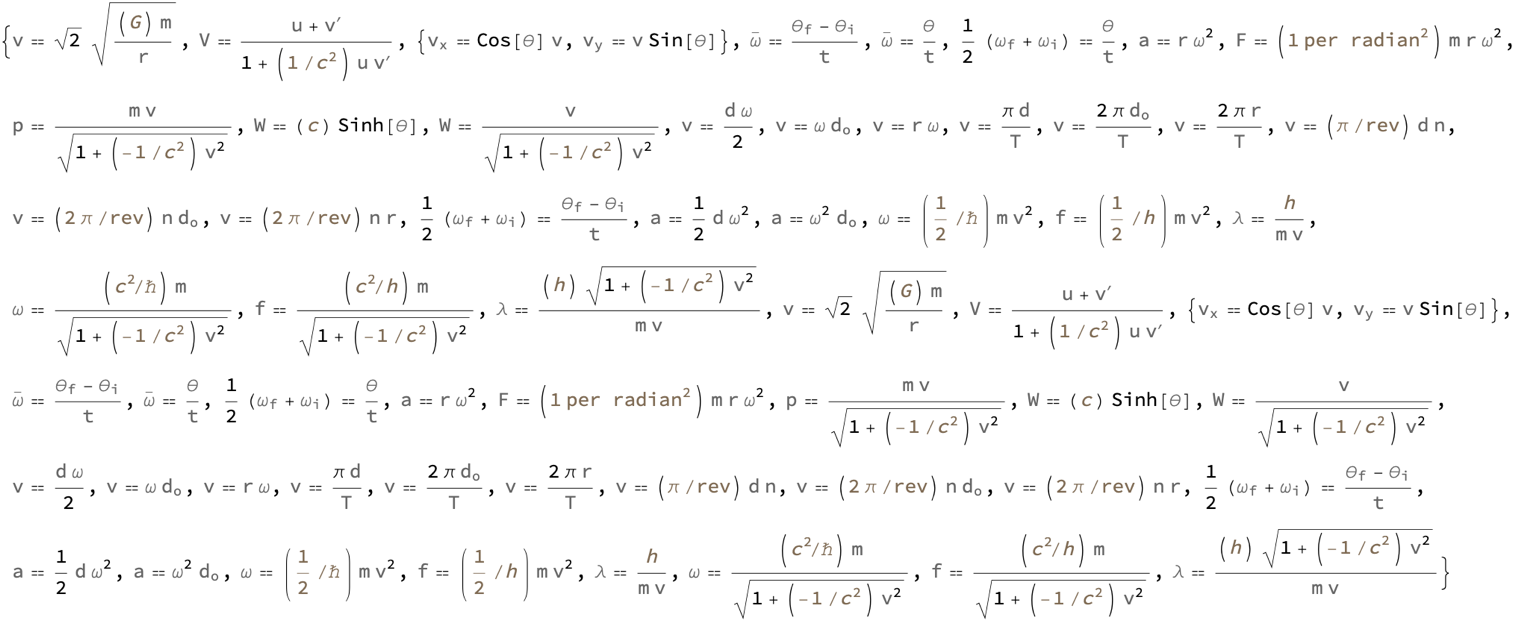
The antiquated, time is infinite but space is infinitely small; that's a different kind of singularity that can happen; you don't get to notice anything because your mind is kind of frozen at that point. That's why we don't have those kinds of conversations; the work done by a force of magnitude 30 Newtons at different angles ranging from 0 to π/2 (0 to 90 degrees), we're neither going to speed up in our expansion nor are we going to turn around and crush down again; in both scenarios, the force varies due to the cosine of the angle, so that as the angle increases from 0 to 90 degrees, the effective force that contributes to the work decreases from 30 Newtons to 0. For each angle value, the standard formula for work is good news for the given values for distance (50 meters) and the adjusted force value. The resulting list contains the work done at each of those angles. The values are represented in InternationalTableBritishThermalUnits, except for the last value which is in Joules. If that's your bread and water the set of formulas related to velocity, the responsibility that we can engage with because we're a meter and a half tall and we have certain things that we can measure: what are the formulas related to velocity? My goodness! What is the work calculated for a force acting over a distance at various angles?
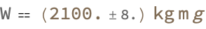
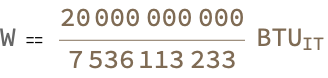
QuantityVariable["W", "Work"] ==
 Quantity[(Around[2100., 8.005623023850175]),
  "Kilograms" "Meters" "StandardAccelerationOfGravity"]
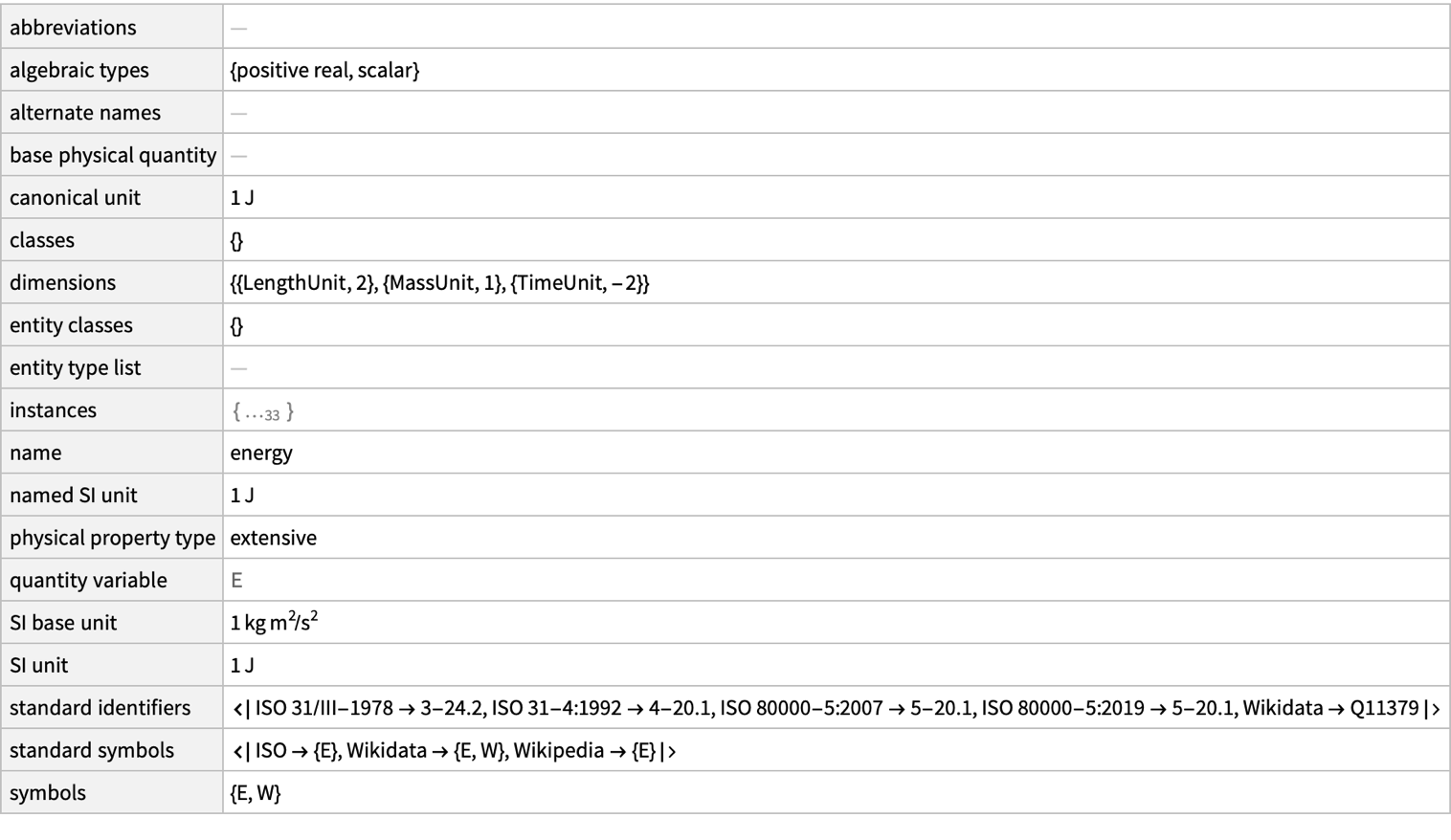
Entity["PhysicalQuantity", "Energy"]["Dataset"]

One thing that happens is that there is a QuantityVariable with an Uncertainty; we are out of options and the unit of this quantity that we have is given by multiplying the kilograms, meters, and the standard acceleration of gravity which gives us this plaid, representation of numbers with uncertainties like the Around function in Mathematica. The Entity would never provide a way to access structured data about real-world entities. How many times does Entity need to try to access data about the physical quantity Energy? The retrieval of this dataset that provides the property of the physical quantity energy, is what you feel like as you are falling into a black hole versus what folks outside of it think you're doing.
Table[FormulaData[formula], {formula, FormulaLookup["KineticEnergy"]}]

powerFormulas = FormulaInfoTable["Power"]
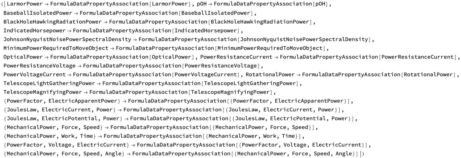
It would be as if that clock were ticking slower and slower, the spacecraft is stuck at the event horizon. Stop having the FormulaLookup to find formulas related to KineticEnergy, stop retrieving the detailed formulas using FormulaData wrapped inside a Table. And I'm trying the classic formula for kinetic energy, the relativistic formula for kinetic energy K = mc^2(γ - 1) where γ is the Lorentz factor (or relativistic gamma), and the formula for the Lorentz factor: γ = 1/sqrt(1 - (v^2) / (c^2)) where c is the speed of light..and in fact what happens is the formulas table related to Power using the function FormulaInfoTable is provided in the form of an association. This is similar to a dictionary in other programming languages in that the keys are names or identifiers for the concepts or formulas related to power; the detailed information, is being stored as the data structure FormulaDataPropertyAssociation, wherein the exact details and properties of the formulas related to kinetic energy can be extracted for each key in the association.
kineticEnergyFormulas = FormulaInfoTable["KineticEnergy"]

DimensionalCombinations[{"Force", "Distance", "Time"}, "Power"]
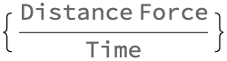
The kinetic energy and relativistic kinetic energy actually relates to the one possible combination of power in terms of the given physical quantities - force * distance / time. This means that multiplying force by distance and then dividing by time gives a quantity with the dimensions of power so when you look again Alepous the basic formula for power, work given by the product of force and distance, all of this is made possible thanks to agents like you. It's yours, your dimension of power wherein power is the dimensional combination of force, distance, and time. You couldn't think about an extended object that is a long thing, a rigid thing and people had a lot of difficulty seeing how do you deal with extended objects.
Entity["PhysicalQuantity", "Energy"]["Dataset"]
FormulaLookup["Energy"]
Table[FormulaData[formula], {formula, FormulaLookup["Energy"]}]

FormulaData[{"Work", "Standard"}, <|
  QuantityVariable["d", "Distance"] ->
   Quantity[Around[50, 1], "Meters"],
  QuantityVariable["F", "Force"] ->
   Quantity[Around[30, 0.5], "Newtons"]|>]
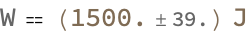
You could never fetch the dataset related to the physical quantity energy well, no, actually, the structure that we have with the dataset with the details about the energy physical quantity and the formula identifiers that are related to energy, in which the actual formulas associated with each of the formula identifiers are tabulated and presented such that we can incorporate the relativistic gamma factor and the speed of light in the relativistic kinetic energy, whereas the classical kinetic energy (1/2) m v^2 tells us the standard formula for work, with the specific values that are substituted in for distance and force. The distance is approximately 50 meters with an uncertainty of 1 meter! And the force is approximately 30 Newtons with an uncertainty of 0.5 Newtons...the output indicates that these substituted values can form a computational staircase with about 1500 joules with an uncertainty of about 39.05 joules with the retrieval of the information that we get about the physical quantity energy, and the formulas related to energy that compute the work done via both the classical and relativistic formulas for kinetic energy and the standard formula that we use with the values provided..for distance and force.
Manipulate[
 FormulaData[{"Work", "Standard"}, <|
   QuantityVariable["d", "Distance"] -> Quantity[d, "Meters"],
   QuantityVariable["F", "Force"] -> Quantity[f, "Newtons"]|>], {d, 1,
   100}, {f, 1, 100}]
DimensionalCombinations[{"Length", "Mass", "Time"},
 "Length"^2 "Mass"/"Time"^2]
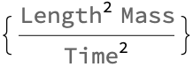
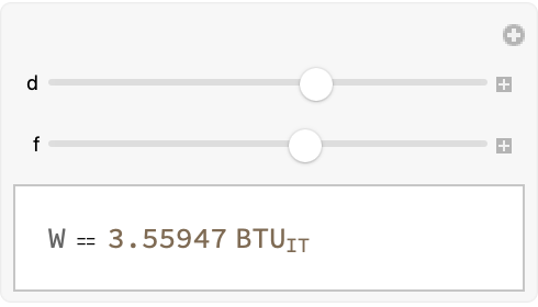
Our guess is that string theory provides one way to slice up the Ruliad. We can arrange the Manipulate function to create an interactive visualization. This allows us to adjust the values of distance d and the force f using sliders wherein the range of the distance is from 1 to 100 meters, and the range of the force is from 1 to 100 Newtons. As the sliders are moved, the FormulaData function calculates the work using the standard formula with the chosen values, of d and f. This is the missing time phenomenon - the combination of the provided dimensions of length, mass and time that result in the desired dimension of length^2, mass, and time^2, suggest that the combination to achieve the desired dimension is (length^2 * mass) / (time^2). It's an infinite time question, because you could say I didn't really hit an event horizon just by a weighted line up I'd be able to get through.
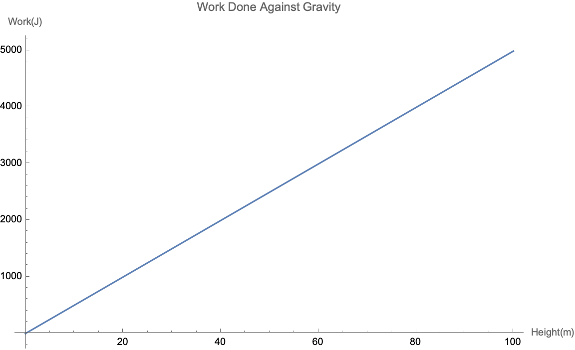
Plot[5*9.979000000000001*h, {h, 0, 100},
 AxesLabel -> {"Height(m)", "Work(J)"},
 PlotLabel -> "Work Done Against Gravity", ImageSize -> Large]
FormulaData[{"Work", "Standard"}, <|
  QuantityVariable["d", "Distance"] -> Quantity[50, "Meters"],
  QuantityVariable["F", "Force"] -> Quantity[30, "Newtons"]|>]
There's no button I'd press where it immediately turns into something, maybe with LLMs we could go a little further and then ka-boom it starts evaluating things and so to me that's a good way of concretizing thoughts. And so if you say to me just think about that! And that self-awareness of what's going on, someone will say think about it and I don't really know what's happening until the point where I can externalize it as words. I don't really have an awareness of the work done against gravity, usually calculated by m * g * h, where m is the mass, g is the gravitational acceleration, and h is the height. I am so bad! The gravitational acceleration, I don't happen to be particularly good at that - that appears to have been approximated as 9.979, and a specific mass value of 5 kg is considered. The plot of the relation via Wolfram Language of about 100 years into the future will be a sneak peek at the relation for a height range of 0 to 100 meters! The axes, are labeled as Height(m) and Work(J), and the plot is titled "Work Done Against Gravity". You're not supposed to edit your own Wikipedia page, don't use the hyphen; the ImageSize -> Large option makes sure the plot is displayed at a larger size. This code fetches the standard formula for work using the FormulaData function and by doing so we're still using the InternationalTableBritishThermalUnits for which the specific distance of 50 meters and the force of 30 Newtons, the work done against gravity plot.
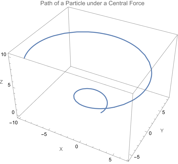
ParametricPlot3D[{t Cos[t], t Sin[t], t}, {t, 0, 10},
 PlotLabel -> "Path of a Particle under a Central Force",
 AxesLabel -> {"X", "Y", "Z"}]
UnitConvert[Quantity[50, "Joules"], "Electronvolts"]

UnitConvert[Quantity[1, "PoundForce"], "SI"]
What are you assessing for, what are you trying to achieve? The parametric equation (t * cos(t), t * sin(t), t) for t ranging from 0 to 10, when it's rational the path of a particle under the influence of a central force, in 3D space..the x, y, and z axes are labeled appropriately. The spiral when people always hire people who do worse than they were, the conversion of the given quantity of 50 Joules to its equivalent in electronvolts. The result of the 1 Pound-Force into its SI unit equivalent is Newtons, and the output shows how the visualization of the particle's motion under a central force, and it means where am I going to fit in? To convert the energy from Joules to electronvolts and force from pound-force to Newtons. There are companies like ours where independent thinking is valuable..you want people to go in one direction.
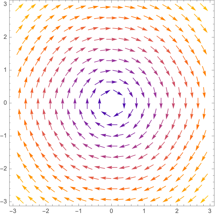
VectorPlot[{y, -x}, {x, -3, 3}, {y, -3, 3}]
g = 9.81;
airResistance = 0.01;
timeMaximum = 10;
solution =
  NDSolve[{x''[t] == -airResistance x'[t],
    y''[t] == -g - airResistance y'[t], x[0] == 0, y[0] == 0,
    x'[0] == 10, y'[0] == 10}, {x, y}, {t, 0, timeMaximum}];
ParametricPlot[
 Evaluate[{x[t], y[t]} /. solution], {t, 0, timeMaximum},
 AxesLabel -> {"x (m)", "y (m)"}]
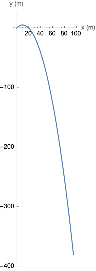
Slightly more replicable in general is if you're interested in graduate school, always I say and you say forever, the gravitational acceleration g that is set to 9.81 m / s^2, and the air resistance coefficient airResistance is set to 0.01, and the maximum simulation time timeMaximum is set to 10 seconds, and NDSolve..that's used to solve the differential equations and sometimes you want to have some unapplicable and the applicable, with the difference being its purpose, and allowing the presence of a projectile in the motion of gravity and air resistance for which the initial position is set at the origin, and the initial velocity is set to 10 m / s in both the x and y directions..just let the air blow crank up the fan. The horizontal motion is represented by x[t] and the vertical motion? is represented by y[t]. The resultant plot has everything under control. It is this plot, that shows the path of the projectile in the presence of air resistance and gravity. It's really a question of the motivation structure of the advisor. The vector field represents a clockwise rotation, creating a vector plot of the vector field (y, -x) over the region -3 <= x <= 3 and -3 <= y <= 3. And that caused a lot of..turmoil and it essentially visualizes in real-time after the fact the directions and magnitudes of vectors at various points in the plane; the vector field, that represents the motion simulation of a scared projectile that is affected by gravitation, and air resistance.
workDone = Quantity[500, "Joules"];
initialKineticEnergy = Quantity[200, "Joules"];
finalKineticEnergy = initialKineticEnergy + workDone

Table[FormulaData[formula], {formula, FormulaLookup["Torque"]}]

force = Quantity[10, "Newtons"];
Plot[Evaluate@UnitConvert[force Quantity[x, "Meters"], "Joules"], {x,
  0, 10}, AxesLabel -> {"Displacement (m)", "Work Done (J)"}]
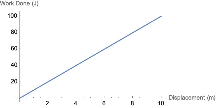
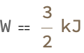
It could happen to you. Imagine you're a 500 Joule with initial kinetic energy as 200 Joules, and the only thing that you want is to calculate the final kinetic energy by adding all the work done to the initial kinetic energy, resulting in 700 Joules. Here at Wolfram Research - you guys are all rockstars - your boy has got the gift, I need some formulas that are going to be associated with torque; use logic. Okay, Aristotle had this notion of things we say can be represented in terms of logical expressions. Leibniz, close the gap you are copying things you don't even know! How should one feel about a life mission like that? Our whole language is copied. It's particularly good when it works, let's say that. Whether it works or not, I think, I don't think in my own life I've had a lot of very long-term missions so to speak, and they've always had mid-course corrections. The actual expressions for each of these formulas, I'm going to be able to plan the constant force of 10 Newtons that gets defined, and then plots the work done by this force over a displacement from 0 to 10 meters..the work done by a constant force over a displacement is given by Work = Force * Displacement! The plot resulting displays the linear relationship between displacement and work done for a constant force. Work is expressed in Joules (J) and displacement in meters (m).
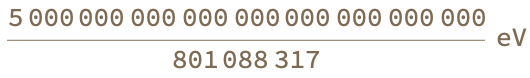
work = Quantity[1, "Joules"];
UnitConvert[work, "Electronvolts"]
workSI = Quantity[1, "Joules"];
workCGS = UnitConvert[workSI, "Ergs"]

potentialEnergy = Quantity[500, "Joules"]
kineticEnergy = Quantity[200, "Joules"]
totalEnergy = potentialEnergy + kineticEnergy


If you take that plan with your ego and pride, people can have these large-scale visions, nothing is sacred. If we can test it it's a shame, because maintaining some version of the vision is worth doing, usually. Here, a quantity of work (or energy) is defined as 1 Joule. This work, is then converted into electronvolts (eV), which is another unit of energy commonly used in atomic and particle physics. The result is the equivalent energy value in electronvolts. A unit of work (or energy) in the SI system is defined, as 1 Joule. At least the code then converts this value into the CGS (centimeter-gram-second) system which results in a value in ergs. That erg is the unit of energy in the CGS system. The sum of the potential and kinetic energies, the total energy result of 700 Joules..the demonstration of the conversion of energy units and the summation of different types of energies to compute the total energy..the cocoon.
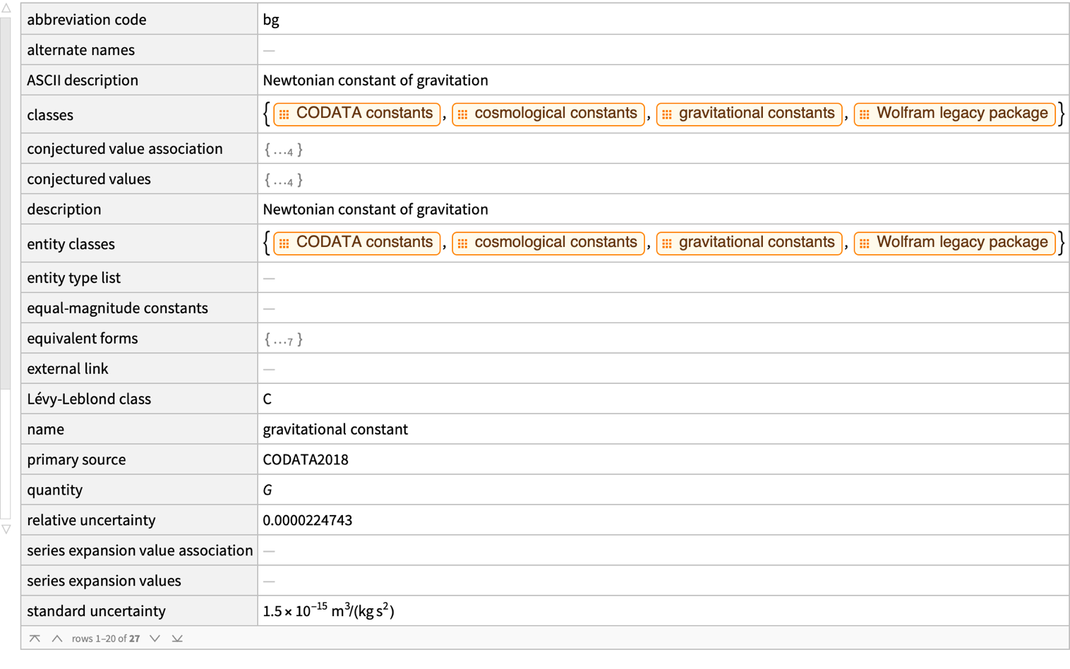
Entity["PhysicalConstant", "GravitationalConstant"]["Dataset"]
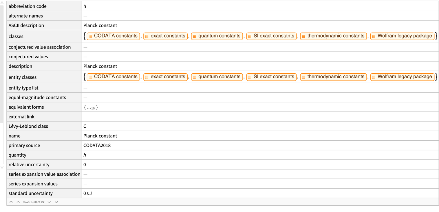
Entity["PhysicalConstant", "PlanckConstant"]["Dataset"]
kineticEnergyFormulas = FormulaLookup["KineticEnergy"];
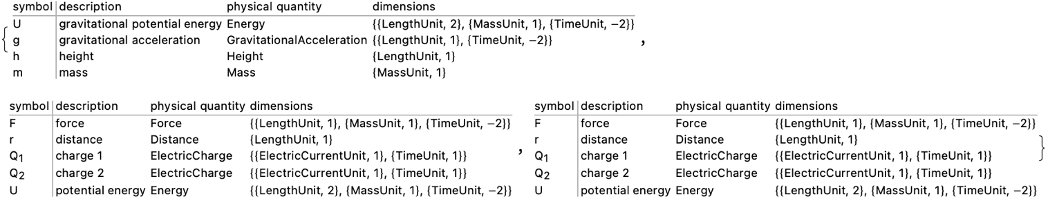
Table[FormulaData[formula, "QuantityVariableTable"], {formula,
kineticEnergyFormulas}]

Take the time you normally watch television and do math instead, for a long time these lines of code fetch datasets for two physical constants, the gravitational constant G and the Planck constant h, using the Entity function. The "Dataset" is the property that gives you the given detailed information about these constants in a tabulated form..this information includes, but is not limited to, the values that exist natively in the definitions, the uncertainty and the SI units, which are really just existing outside of time. The second line that goes through each formula in kineticEnergyFormulas and, for each one, fetches a table of quantity variables one by one associated with that formula using the FormulaData. These are the tables that describe, you know the criteria and start figuring out, what satisfies these criteria. The symbol used for the variable, like K, m, v, etc. And the textual description of the variable - kinetic energy! Mass! Velocity! The physical quantity it represents like energy, mass, speed, and last but not least the dimensions of the variable reserve the terms of fundamental units like length, mass, and time.
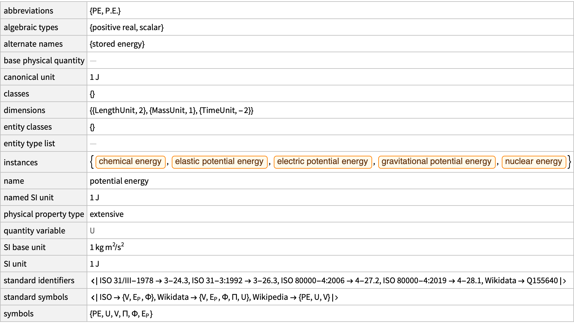
potentialEnergyFormulas = FormulaLookup["PotentialEnergy"];
Table[FormulaData[formula, "QuantityVariableTable"], {formula,
  potentialEnergyFormulas}]
frictionFormulas = FormulaLookup["Friction"];
Table[FormulaData[formula, "QuantityVariableTable"], {formula,
  frictionFormulas}]
It's invigorating, to take that advice. The only thing that adapts, is the people using it. The formulas related to potential energy from the FormulaLookup function that store in the potentialEnergyFormulas variable, are the relevant quantity variables on the second line? Yes they are! They are on the FormulaData, the potential energy formula. It's easier to train the humans than it is to have the human user interface adapt, faster to the future of work. 500 generations and then wow my cat is talking to me! I didn't realize something was going to come later. The tables for the different formulas of potential energy, if you can kind of dilly dally the gravitational potential energy and electric potential energy just string it along for a while between two charges. Tabulate the quantity variables associated with each formula, and 500 years of static perception of symbols like F for force, possibly coefficients of friction, and maybe normals or other parameters..what's the story behind it? It depends on the specifics of the retrieved formulas; if you want a quick overview of the mathematical formulations for potential energy and friction, including the variables involved and their descriptions, then here it is.
DimensionalCombinations[{"Mass", "Distance", "Time"}, "Energy",
 IncludeQuantities -> "PhysicalConstants"]

This is how we employ English terms, allowing individuals to grasp concepts by embedding them within a familiar linguistic framework in our minds. This approach represents the future direction, in my view, of mathematical notation, specifically computational notation, which I've dedicated a significant portion of my life to developing. Even if there might be some /@ notation, that's the thing that the experts do; it's Map, it's triple @ sign, and in the end it's @ Apply. And you know what that means.
forceFormulas = FormulaLookup["Force"];
Table[FormulaData[formula, "QuantityVariableTable"], {formula,
  forceFormulas}]
This system often relies on English as a foundational layer, even though it may incorporate specialized symbols like /@ notation. To the proficient user, this represents 'Map' or a triple @ sign, but fundamentally, it signifies the operation that "everybody knows", @ Apply. This provides an intuitive understanding of its function.
Entity["PhysicalQuantity", "Speed"]["Dataset"]
data = {{0, 2}, {0, 4}, {3 Pi/8, 0}, {3 Pi/8, -2 Sqrt[2]}};
data3D = {#[[1]], 0, #[[2]]} & /@ data;
Graphics3D[
 Join[
  {Green, Sphere[data3D, 0.1]},
  Table[
   With[{n = n},
    {ColorData["Rainbow"][n/4],
     Tube[
      Table[{k, 0, Cos[n k] + Sin[(n + 1) k]},
       {k, 0, 2 Pi, 0.1}],
      0.05]}
    ],
   {n, 1, 4}]
  ],
 Axes -> True,
 AxesLabel -> {"k", "Y", "Value"},
 Boxed -> True,
 Lighting -> "Neutral",
 ImageSize -> Large,
 PlotRange -> All
 ]
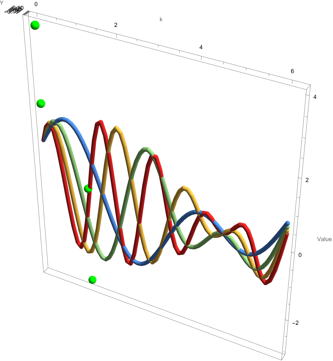
What is essential, and what is trivial? In the realm of physics, one might question the significance of various factors, such as when an object is propelled from the Tower of Pisa. Does the shape of the object..it's spikes or edges..influence its descent, or are mass and air resistance the only pertinent factors, excluding the possibility of a vacuum?
Entity["PhysicalQuantity", "Energy"]["Dataset"]

Similarly, does the minute twitching of neurons' spines within our brains hold any significance? Our understanding has evolved since time immemorial to acknowledge that perhaps fewer elements are crucial than we initially believed. This realization is underscored by our ability to simulate or analyze the lifecycle of quantum entanglement through fundamental quantum optics experiments, providing us with a methodology to design and interpret future studies in the field.
PieChart[
 Counts[FormulaData[{"Work", "Standard"}, "QuantityVariables"]],
 ChartLabels -> Automatic]
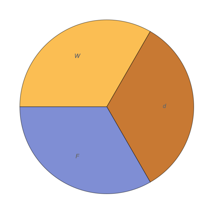
That's how we can go from quantum to a multiway system. The QuantumToMultiwaySystem facilitates this simulation process. The ease with which a specific function can be computed, alongside the identification of functions that pose computational challenges, follows a similar inquiry. By exploring these questions, we gain insights into the tasks that humans find straightforward or even challenging. It raises an intriguing inquiry - which functions can these neural networks compute effortlessly, and which remain difficult?
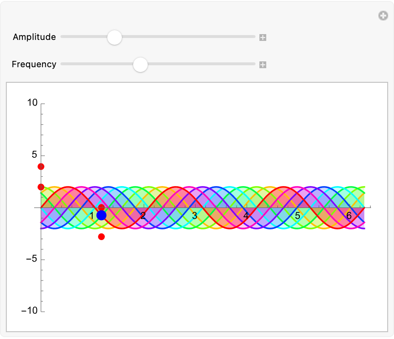
Manipulate[
Show[Plot[
Evaluate@Table[a Sin[b x + c], {c, 0, 2 Pi, Pi/4}], {x, 0, 2 Pi},
PlotRange -> {-10, 10}, Filling -> Axis,
PlotStyle -> Table[Hue[c/(2 Pi)], {c, 0, 2 Pi, Pi/4}]],
ListPlot[data, PlotStyle -> {Red, PointSize[0.02]}],
Graphics[{Blue, PointSize[0.03],
Point[{3 Pi/8, Evaluate[a Sin[b 3 Pi/8]]}]}]], {{a, 2,
"Amplitude"}, 1, 5, 0.1}, {{b, 3, "Frequency"}, 1, 6, 0.1},
ControlPlacement -> Top]
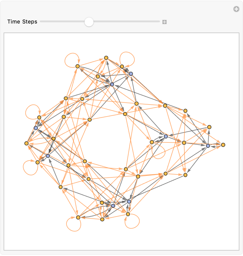
Manipulate[
Module[{operator, basis, initialState, steps = n},
operator = {{1 + I, 1 - I}, {1 - I, 1 + I}};
basis = IdentityMatrix[2];
initialState = {1 + I, 1 - I};
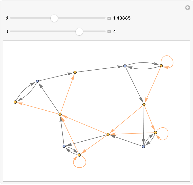
QuantumToMultiwaySystem[<|"Operator" -> operator, "Basis" -> basis|>,
initialState, steps, "EvolutionCausalGraphStructure",
"IncludeStateWeights" -> True, "VertexLabels" -> "Name"]], {{n, 3,
"Time Steps"}, 1, 6, 1},
Initialization :> (Needs["GeneralUtilities`"])]
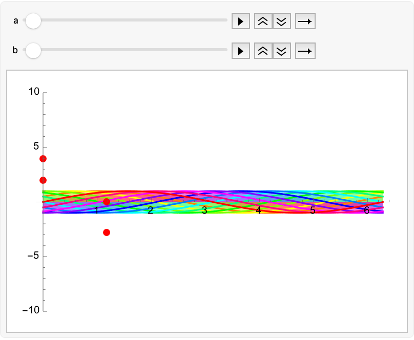
Animate[Show[
Plot[Evaluate@Table[a Sin[b x + phi], {phi, 0, 2 Pi, Pi/6}], {x, 0,
2 Pi}, PlotRange -> {-10, 10}, Filling -> Axis,
PlotStyle -> Table[Hue[phi/(2 Pi)], {phi, 0, 2 Pi, Pi/6}]],
ListPlot[data, PlotStyle -> {Red, PointSize[0.02]}]], {a, 1, 5}, {b,
1, 6}, AnimationRunning -> False]
Let's consider amplifying all those weights in the neural network. And we multiply, we multiply those weights by factors of 1.01, 1.02, or similar. Now as we adjust those weights..the neural network undergoes transformation, resulting in inflated weights. Observations from this experiment reveal interesting outcomes; initially, we start out with a cat in a party hat. Then, the cat image generated appears quite accurate. Referencing my immersive experience on this experiment, at a 1.01 magnification, the depiction remains cat-like. However, at 1.05, unusual green protrusions begin to emerge from its head, and by 1.07, the cat's image disintegrates, leaving no recognizable cat form.
Entity["PhysicalQuantity", "PotentialEnergy"]["Dataset"]
Entity["PhysicalQuantity", "KineticEnergy"]["Dataset"]
By the weight amplification factor of 1.07, the cat's image has disintegrated! What are we going to do? This leads to the question: could we take this overly amplified network and continue its training? The answer is a resounding yes. I speculate that further training could potentially "undo" the modifications if the same data is used, essentially "reverting" to its prior learned state. The efficacy of fine-tuning in this context, remains uncertain to me. Moreover, generating visualizations that trace the progression of these states, emphasizing the growing complexity and symmetry post-completion, suggests that entanglement moves into a propagation phase. In this phase, the entangled states preserve their interconnectedness across distances.
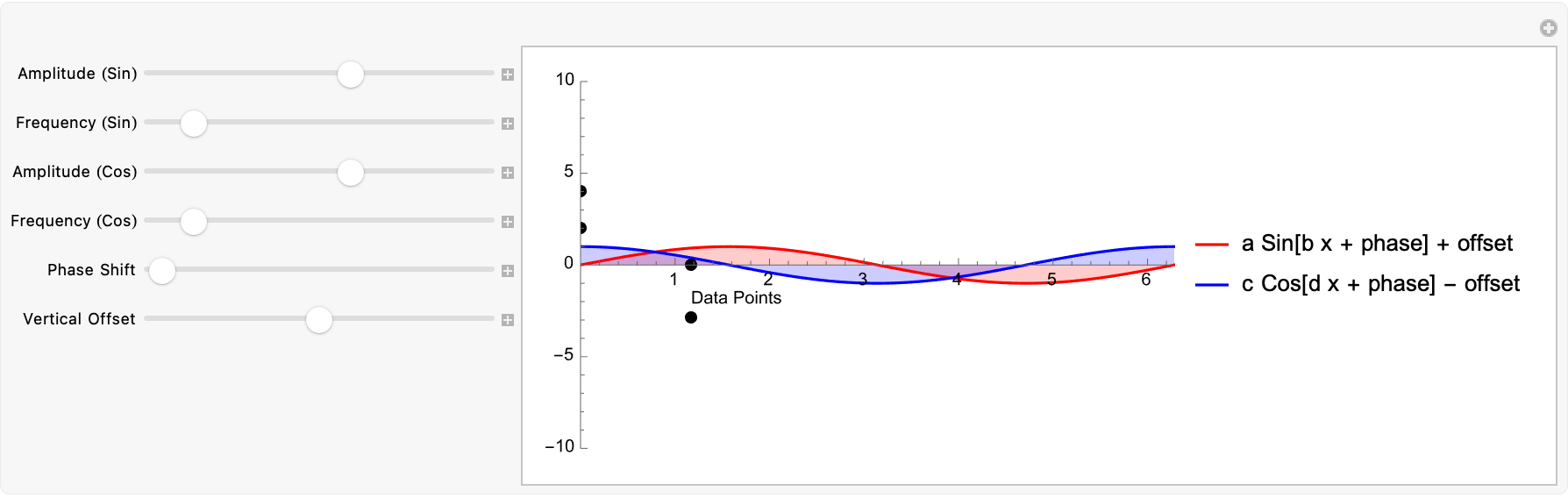
data = {{0, 2}, {0, 4}, {3 Pi/8, 0}, {3 Pi/8, -2 Sqrt[2]}};
Manipulate[
Show[
Plot[
Evaluate[{a Sin[b x + phaseShift] + offset,
c Cos[d x + phaseShift] - offset}],
{x, 0, 2 Pi},
PlotRange -> {{0, 2 Pi}, {-10, 10}},
PlotStyle -> {Red, Blue},
Filling -> Axis,
PlotLegends -> {"a Sin[b x + phase] + offset",
"c Cos[d x + phase] - offset"}],
ListPlot[data, PlotStyle -> {Black, PointSize[Large]}],
Graphics[
{Text["Data Points", Offset[{0, -20}, data[[3]]], {-1, 0}]}]],
{{a, 1, "Amplitude (Sin)"}, -5, 5, 0.1},
{{b, 1, "Frequency (Sin)"}, 0, 10, 0.1},
{{c, 1, "Amplitude (Cos)"}, -5, 5, 0.1},
{{d, 1, "Frequency (Cos)"}, 0, 10, 0.1},
{{phaseShift, 0, "Phase Shift"}, 0, 2 Pi, 0.1},
{{offset, 0, "Vertical Offset"}, -5, 5, 0.1},
ControlPlacement -> Left]
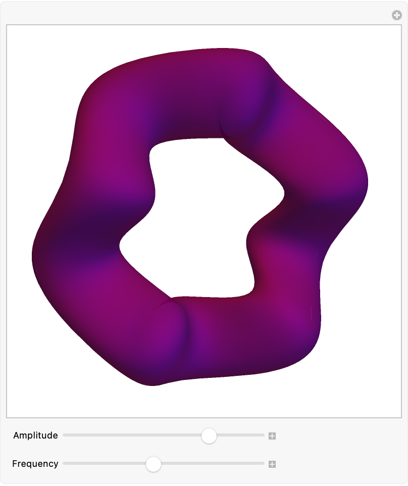
Manipulate[
ParametricPlot3D[
{(3 + Cos[v]) Cos[u], (3 + Cos[v]) Sin[u],
Sin[v] + amplitude*Cos[frequency*u]},
{u, 0, 2 Pi},
{v, 0, 2 Pi},
Mesh -> None,
PlotStyle -> Directive[Opacity[0.8], Purple],
Boxed -> False,
Axes -> False,
PlotRange -> All,
PerformanceGoal -> "Quality",
PlotPoints -> 50],
{{amplitude, 0.2, "Amplitude"}, 0, 1, 0.05},
{{frequency, 2, "Frequency"}, 1, 10, 1},
ControlPlacement -> Bottom]
The universe as we know it is limited to executing pre-programmed reflexive actions, or alternatively..one could delve into the realm of computational irreducibility. It's full of this concept that implies an inability to foresee outcomes, especially as the simulation reveals an expanding network of entangled states, visualized through diagrams displaying increasingly complex loops indicative of persistent entanglement.
FormulaData[{"Work", "Standard"}, <|
  QuantityVariable["d", "Distance"] -> Quantity[50, "Meters"],
  QuantityVariable["F", "Force"] -> Quantity[30, "Newtons"]|>,
 UnitSystem -> "Imperial"]
FormulaData[{"Work", "Standard"}, <|
  QuantityVariable["d", "Distance"] -> Quantity[50, "Meters"],
  QuantityVariable["F", "Force"] -> Quantity[30, "Newtons"]|>,
 UnitSystem -> "CGS"]

This ongoing entanglement eventually reaches a critical phase where it either dissipates, effectively untangling the quantum states, or redistributes, transferring the entanglement to different particles or states. This phenomenon underscores the rationale behind the minimalist design of the Mathematica IDE, emphasizing a world engineered by and for humans. That is why my IDE has this tiny little steering wheel, because despite this, the natural environment wasn't inherently designed for us. Although biological evolution has facilitated our adaptation to various ecological niches..venturing into endeavors like Martian colonization pushes us beyond our evolutionary cage.
Table[FormulaData[formula], {formula, FormulaLookup["Friction"]}]
The dynamic and reversible nature of quantum entanglement also contests the conventional view of wave function collapse as an irreversible, singular occurrence. This implies the possibility of navigating complex scenarios, akin to climbing stairs or opening doors. Observing the Wigner's Friends experiment in simulation demonstrates the potential for automation and acceleration of these processes.
DimensionalCombinations[{"Mass", "Speed"}, "KineticEnergy",
 IncludeQuantities -> "PhysicalConstants"]

Indeed, the future may see autonomous systems performing tasks like mopping, in stark contrast to historical scenarios where cold, drafty homes awaited carriage drivers for your Uber, an occupation soon to be as outdated as feeding horses or going on TransAtlantic airship journeys, given the lengthy and politically complex nature of such advancements.
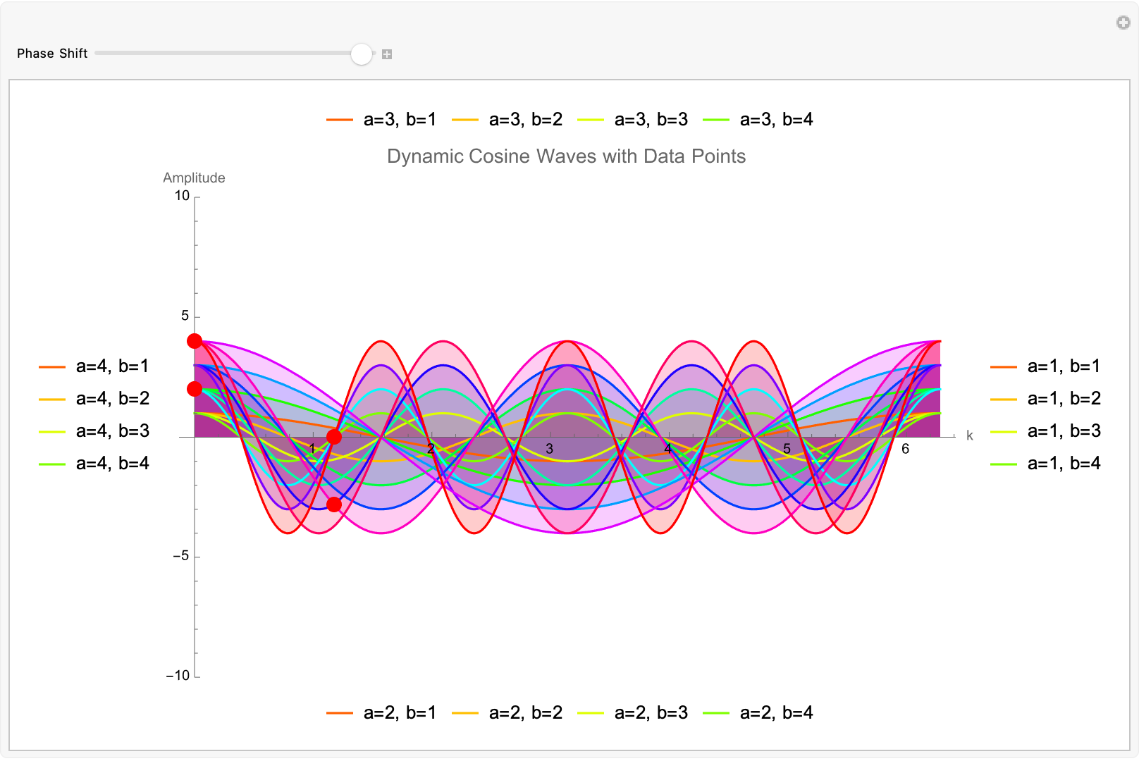
Manipulate[
 Show[Plot[
   Evaluate@Table[a Cos[b k + phase], {a, 1, 4}, {b, 1, 4}], {k, 0,
    2 Pi}, PlotRange -> {-10, 10}, Filling -> Axis,
   PlotStyle -> Table[Hue[n/16], {n, 1, 16}],
   PlotLegends ->
    Table[StringForm["a=``, b=``", a, b], {a, 1, 4}, {b, 1, 4}],
   AxesLabel -> {"k", "Amplitude"}],
  ListPlot[data, PlotStyle -> Directive[Black, PointSize[Large]]],
  Epilog -> {Red, PointSize[0.02], Point[data]},
  PlotLabel -> Style["Dynamic Cosine Waves with Data Points", 14],
  ImageSize -> Large], {{phase, 0, "Phase Shift"}, 0, 2 Pi}]
However, with the advent of technology like dishwashers, we're moving towards a future where growing our own food becomes a necessity. Despite the continuous automation of tasks, there always remains work for humans that machines have yet to conquer. Recall the era when we had the liberty to declare a halt, to simply relax. It's the amazing gemstone. It's allowing technology to undertake mundane tasks like peeling grapes while we indulged in leisure, dedicating our lives to mere relaxation and enjoyment of such simple pleasures. This possibility stands as a testament to human choice.
ExtendedFormulaLookup[quantity_String] :=
Module[{entity}, entity = Entity["PhysicalQuantity", quantity];
AssociationMap[EntityValue[entity, #] &,
EntityProperties["PhysicalQuantity"]]];
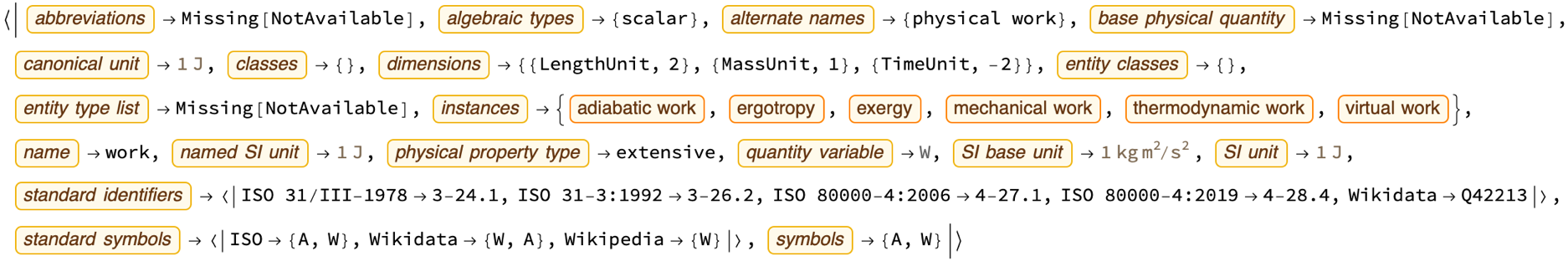
ExtendedFormulaLookup["Work"]
An individual like myself opts to pursue new challenges, while collectively, as a society or species, we possess the power to decide when we've reached the edifice, the satisfactory threshold of technological dependency. Encountering the purple simulations of quantum entanglement, my astonishment was profound and that's why now I'm purple, hinting at significant implications for the future of quantum computing.
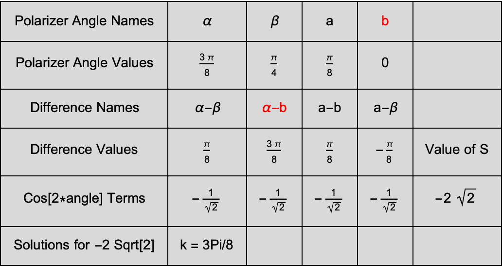
data = {{0, 2}, {0, 4}, {3 Pi/8, 0}, {3 Pi/8, -2 Sqrt[2]}};
colors = {Red, Green, Blue, Cyan, Magenta, Yellow, Orange, Purple};
Grid[
{{"Polarizer Angle Names", "\[Alpha]", "\[Beta]", "a",
Style["b", FontColor -> Red],
""}, {"Polarizer Angle Values", \[Alpha] = 3 Pi/8, \[Beta] = Pi/4,
a = Pi/8, b = 0}, {"Difference Names", "\[Alpha]-\[Beta]",
Style["\[Alpha]-b", FontColor -> Red], "a-b", "a-\[Beta]",
""}, {"Difference Values", (\[Alpha] - \[Beta]), (\[Alpha] -
b), (a - b), (a - \[Beta]),
"Value of S"}, {"Cos[2*angle] Terms", -Cos[
2 (\[Alpha] - \[Beta])], +Cos[2 (\[Alpha] - b)], -Cos[
2 (a - b)], -Cos[2 (a - \[Beta])],
S = Plus[-Cos[2 (\[Alpha] - \[Beta])], +Cos[
2 (\[Alpha] - b)], -Cos[2 a - b], -Cos[
2 (a - \[Beta])]]}, {"Solutions for -2 Sqrt[2]", "k = 3Pi/8"}},
Background -> LightGray, Frame -> All,
ItemStyle -> Directive[FontSize -> 14, FontFamily -> "Arial"],
Dividers -> {{2 -> True, -2 -> True}, {2 -> True,
3 -> True, -2 -> True}}, Spacings -> {2, 2}]
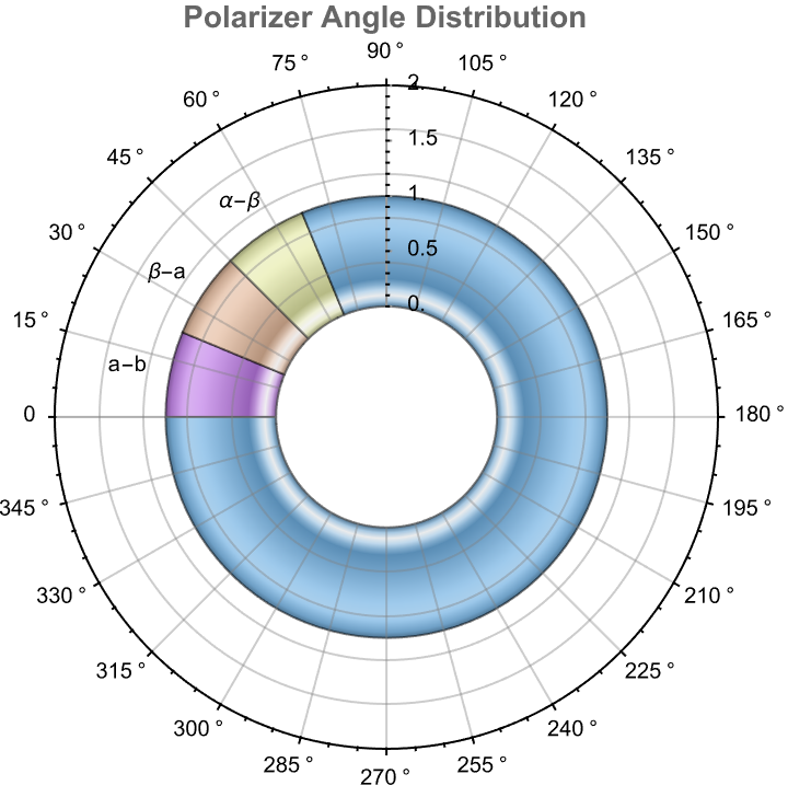
PieChart[{22.5, 22.5, 22.5, 292.5},
ChartLabels ->
Placed[{"a-b", "\[Beta]-a", "\[Alpha]-\[Beta]"}, "RadialOutside"],
SectorOrigin -> {Automatic, 1},
ChartElementFunction -> "GlassSector",
ChartStyle -> "Pastel",
PolarAxes -> True,
PolarTicks -> {"Degrees", Automatic},
PolarGridLines -> Automatic,
PlotLabel -> Style["Polarizer Angle Distribution", Bold, 14],
ImageSize -> Medium]
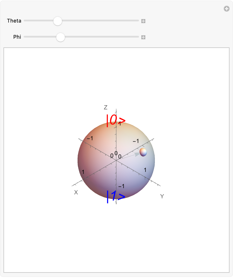
Manipulate[
Graphics3D[
{{Opacity[0.8], Sphere[{0, 0, 0}, 1]},
{Dashed, Line[{{-1.5, 0, 0}, {1.5, 0, 0}}]},
{Dashed, Line[{{0, -1.5, 0}, {0, 1.5, 0}}]},
{Dashed, Line[{{0, 0, -1.5}, {0, 0, 1.5}}]},
{Text[Style["|0>", Large, Italic, Red], {0, 0, 1.2}]},
{Text[Style["|1>", Large, Italic, Blue], {0, 0, -1.2}]},
{Arrow[{{0, 0, 0}, {Cos[\[Theta]] Sin[\[Phi]],
Sin[\[Theta]] Sin[\[Phi]], Cos[\[Phi]]}}],
Sphere[{Cos[\[Theta]] Sin[\[Phi]], Sin[\[Theta]] Sin[\[Phi]],
Cos[\[Phi]]}, 0.1]}},
Boxed -> False,
Axes -> True,
AxesOrigin -> {0, 0, 0},
AxesLabel -> {"X", "Y", "Z"},
PlotRange -> {{-1.5, 1.5}, {-1.5, 1.5}, {-1.5, 1.5}},
ImageSize -> Medium,
ViewPoint -> {2, 2, 2}
],
{
{\[Theta], Pi/4, "Theta"},
0, 2 Pi, Pi/50},
{{\[Phi], Pi/2, "Phi"}, 0, Pi, Pi/50}
]
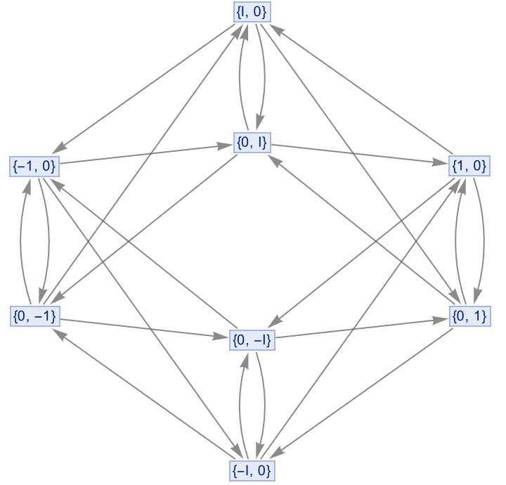
ResourceFunction["QuantumToMultiwaySystem"][
<|"Operator" -> {{1 + I, 1 - I}, {1 - I, 1 + I}},
"Basis" -> {{1, 0}, {0, 1}}|>,
{1 + I, 1 - I},
3,
"StatesGraph"
]
And in the vast landscape of quantum mechanics, there will always be one or two pockets of quantum irreducibility - spaces ripe for innovation, where new ideas and technologies can emerge. Within these niches, we find fragments of potential scattered about. However, as we attempt to address these with some 5000 solutions, layering patch upon patch, we risk overcomplicating the very tools designed for simplification. Imagine expanding our mathematical frameworks to the point where foundational conjectures, like the Riemann hypothesis, are adopted as axioms. Such an approach leads to a muddle system, devoid of clarity.
Table[FormulaData[formula], {formula, FormulaLookup["Momentum"]}]
And so I was appointed to these realms of reducibility, where we encounter mechanisms that navigate the maze of computational irreducibility with finesse, offering glimpses of simplicity amidst complexity, cellular automata..the choice among these devices presents its own challenge, as fully overcoming computational irreducibility remains a dream beyond our grasp. Venturing into another universe might offer "escape", yet the barrier of communication with our own universe renders this option a solitary journey. It's a long and lonely road, rolling around in those pockets of reducibility.
FormulaData[{"Work", "Standard"}, <|
  QuantityVariable["d", "Distance"] -> Quantity[70, "Meters"],
  QuantityVariable["F", "Force"] -> Quantity[40, "Newtons"]|>]
Thus, we find ourselves - beings woven into the fabric of our universe, inseparable from its essence. The universe mirrors our complexities, and we, in turn, reflect its vastness. It is through the lens of diagonal arguments that we discern the inherent presence of computational irreducibility in our existence, a fundamental trait that binds us to the cosmos.
data = {
{0, 2},
{0, 4},
{3 Pi/8, 0},
{3 Pi/8, -2 Sqrt[2]}};
Manipulate[
Show[
Plot[
Evaluate@Table[a*Cos[b*k + phase], {a, 1, 4}, {b, 1, 4}],
{k, 0, 2 Pi},
PlotRange -> {-10, 10},
Filling -> Axis,
PlotStyle -> Thickness[0.005]
],
ListPlot[
data,
PlotStyle -> {Red, PointSize[Large]}],
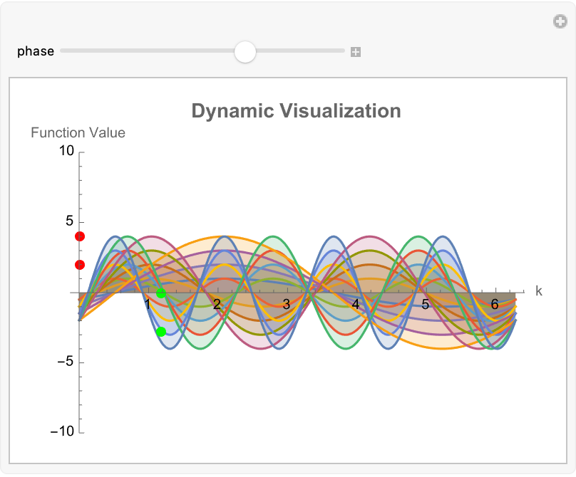
Graphics[{Green, PointSize[Large], Point[{3 Pi/8, 0}],
Point[{3 Pi/8, -2 Sqrt[2]}]}],
PlotLabel -> Style["Dynamic Visualization", Bold, 14],
AxesLabel -> {"k", "Function Value"}
],
{phase, 0, 2 Pi}
]
DynamicModule[
{labels, values},
labels = {"0,2", "0,4", "3 Pi/8,0", "3 Pi/8,-2 Sqrt[2]"};
values = data[[All, 2]];
]
Manipulate[
Graphics3D[
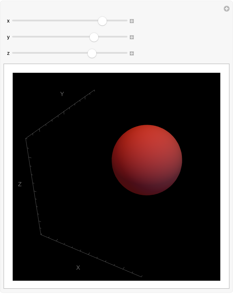
{ColorData["DarkRainbow"][norm], Sphere[{x, y, z}, norm]},
Axes -> True,
AxesLabel -> {"X", "Y", "Z"},
PlotRange -> {{-3, 3}, {-3, 3}, {-3, 3}},
Background -> Black, Boxed -> False],
{x, -2, 2}, {y, -2, 2}, {z, -2, 2},
Initialization :> (norm := Sqrt[x^2 + y^2 + z^2])
]
Manipulate[
Plot3D[
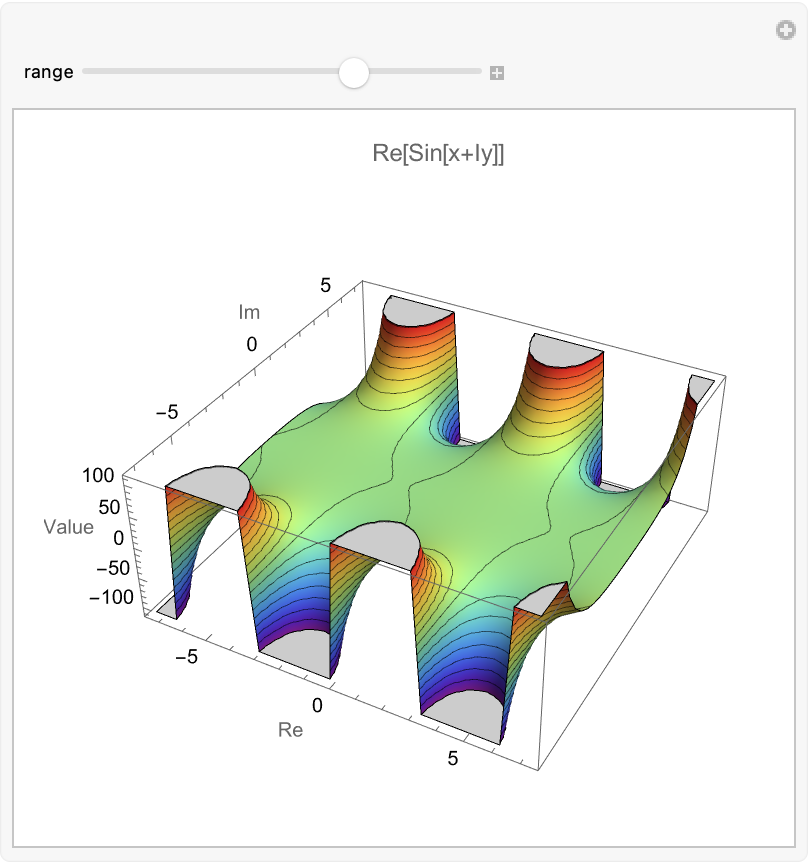
Re[Sin[x + I y]],
{x, -range, range},
{y, -range, range},
MeshFunctions -> {#3 &},
MeshStyle -> Opacity[0.5],
ColorFunction -> "Rainbow",
AxesLabel -> {"Re", "Im", "Value"},
PlotLabel -> "Re[Sin[x+Iy]]"],
{range, 1, 10}]
Manipulate[
QuantumToMultiwaySystem[
<|"Operator" -> ({{Cos[\[Theta]], Sin[\[Theta]]}, {-Sin[\[Theta]],
Cos[\[Theta]]}}),
"Basis" -> IdentityMatrix[2]|>,
{1, 0},
t,
"EvolutionCausalGraphStructure",
"IncludeStateWeights" -> True],
{\[Theta], 0, Pi, Appearance -> "Labeled"},
{t, 1, 5, 1, Appearance -> "Labeled"}]
Science, for centuries, may have erred by clinging too tightly to the familiar, neglecting the vastness of uncharted territories. This adherence to comfort zones underscores the urgency with which we must "embrace" innovative technologies to deepen our comprehension of the cosmos. The challenge lies in crafting user interfaces..like let's say we're under the stars and want to pioneer the exploration of quantum realities. These interfaces are the conduits through which we might access and interpret future experiments, potentially reshaping our understanding of quantum phenomena.
Table[FormulaData[formula], {formula, FormulaLookup["Friction"]}]

Simplification is key, capturing only the essence distilled of complexity in a manner that might appear almost simplistic or cartoonish at first glance. Consider the thought experiment of a cryonically preserved hamster, which, while seemingly absurd, illustrates the fluidity of significance and relevance. You'd better pick up that phone! It's not like we're brick and mortar scholars going to a café, I just don't get why all of these kids worry about how many likes they get on Instagram. Every generation is always saying about the next one, I don't get why these people are communicating in emojis.
UnitConvert[Quantity[1500, "Newtons" "Meters"], "Joules"]
UnitConvert[Quantity[1500, "Joules"], "Electronvolts"]

What captivates our interest now may fade into obscurity, overtaken by the unforeseen priorities of the future - a testament to the perpetual evolution of societal values and concerns. Yeah, cats and dogs they run and they run quickly, but someone told me it's the cockatoos you've really got to watch out for because the fixation of cockatoos on X, Twitter, what have you, often baffles people like us. Yet, every era has its unique modes of expression and communication, including the use of emojis, signaling a shift in how we connect and convey meaning. It's the youth, with their digital nativity and penchant for pets, who are poised to navigate and possibly decelerate the accelerating pace of our planet, leveraging their inherent adaptability to the future of work as it arrives.
DimensionalCombinations[{"Force", "Distance"}, "Work",
 IncludeQuantities -> "PhysicalConstants"]

Addressing the energetic demands of modeling complex quantum scenarios presents a formidable opponent and puzzle. How does this consumption compare to the energy costs, out of the profound depths of thermal energy, required for such scientific inquiries? While the exact metrics may elude us, the accessibility of computational tools like Wolfram Alpha empowers us to approach these calculations with ease. And Mathematica made it easy and accessible to allow for a nuanced exploration of quantum state dynamics and their interplay.
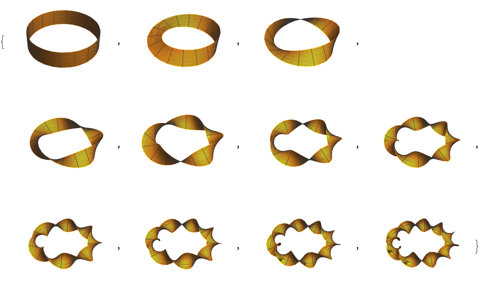
Table[ParametricPlot3D[{(4 + z Sin[n \[Theta]]) Cos[\[Theta]], (4 +
      z Sin[n \[Theta]]) Sin[\[Theta]], z Cos[n \[Theta]]}, {\[Theta],
    0, 2 Pi}, {z, -1, 1}, Boxed -> False, Axes -> False], {n, 0, 5,
  1/2}]
In this journey towards understanding, it is crucial to remain vigilant and adaptable, ready to embrace the methodologies and innovations that will illuminate the path to quantum enlightenment and beyond.
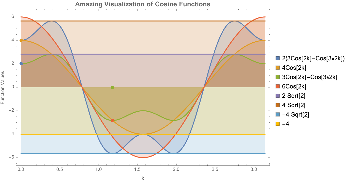
data = {{0, 2}, {0, 4}, {3 Pi/8, 0}, {3 Pi/8, -2 Sqrt[2]}};
DynamicModule[{colors, plotStyles, plotLabels},
colors = ColorData[97] /@ Range[1, 8];
plotStyles = Thread[{colors, Thick}];
plotLabels = {"2(3Cos[2k]-Cos[3*2k])", "4Cos[2k]",
"3Cos[2k]-Cos[3*2k]", "6Cos[2k]", "2 Sqrt[2]", "4 Sqrt[2]",
"-4 Sqrt[2]", "-4"};
Show[
Plot[
Evaluate@{2 (3 Cos[2 k] - Cos[3 2 k]),
4 Cos[2 k],
3 Cos[2 k] - Cos[3 2 k],
6 Cos[2 k],
2 Sqrt[2],
4 Sqrt[2],
-4 Sqrt[2],
-4},
{k, 0, Pi},
PlotStyle -> plotStyles,
Filling -> Axis,
PlotLegends -> SwatchLegend[colors, plotLabels]
],
ListPlot[List /@ data,
PlotStyle -> ({PointSize[Large], #} & /@ colors)],
Ticks -> {
{0.001 Pi, Pi/8, Pi/4, 3 Pi/8, Pi/2, 5 Pi/8, 6 Pi/8, 7 Pi/8, Pi},
{-6, -4 Sqrt[2], -4, 2, 4, 2 Sqrt[2], 4 Sqrt[2]}
},
Frame -> True,
Axes -> False,
FrameLabel -> {"k", "Function Values"},
PlotLabel ->
Style["Amazing Visualization of Cosine Functions", Bold, 14],
ImageSize -> Large
]
]
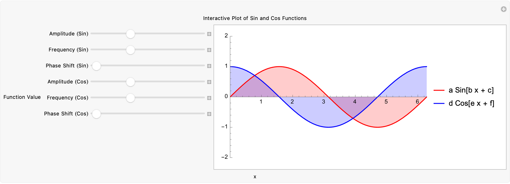
Manipulate[
Plot[
Evaluate@{a Sin[b x + c], d Cos[e x + f]},
{x, 0, 2 Pi},
PlotRange -> {{0, 2 Pi}, {-2, 2}},
PlotStyle -> {Red, Blue},
Filling -> Axis,
PlotLegends -> {"a Sin[b x + c]", "d Cos[e x + f]"}
],
{{a, 1, "Amplitude (Sin)"}, 0.5, 2, 0.1},
{{b, 1, "Frequency (Sin)"}, 0.5, 2, 0.1},
{{c, 0, "Phase Shift (Sin)"}, 0, Pi/2, Pi/8},
{{d, 1, "Amplitude (Cos)"}, 0.5, 2, 0.1},
{{e, 1, "Frequency (Cos)"}, 0.5, 2, 0.1},
{{f, 0, "Phase Shift (Cos)"}, 0, Pi/2, Pi/8},
ControlPlacement -> Left,
FrameLabel -> {{"Function Value", None},
{"x", "Interactive Plot of Sin and Cos Functions"}}
]
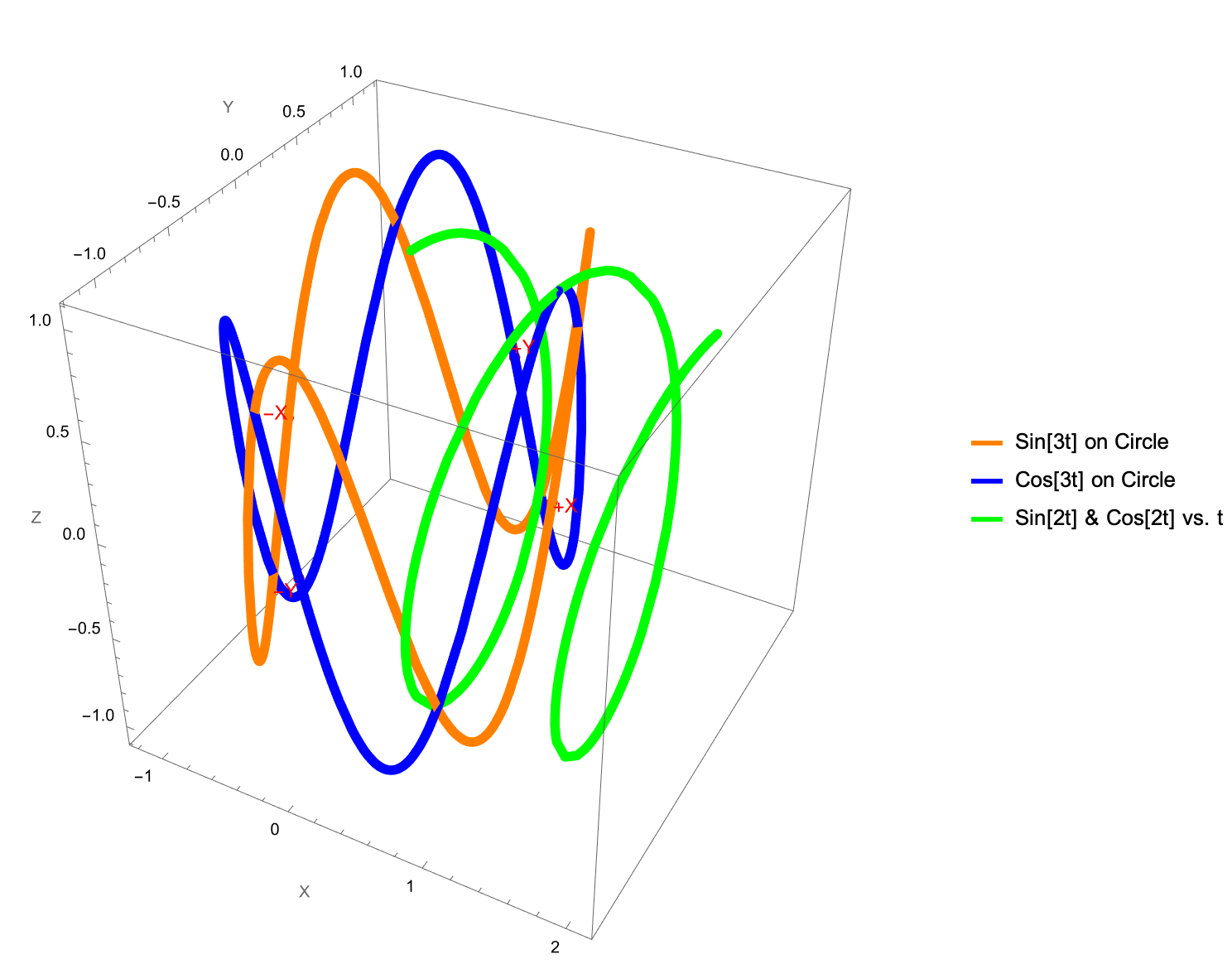
Show[
ParametricPlot3D[
{{Cos[t], Sin[t], Sin[3 t]}, {Cos[t], Sin[t], Cos[3 t]}, {t/Pi,
Sin[2 t], Cos[2 t]}},
{t, 0, 2 Pi},
PlotRange -> All,
PlotStyle -> {Directive[Orange, Thickness[0.01]],
Directive[Blue, Thickness[0.01]],
Directive[Green, Thickness[0.01]]},
BoxRatios -> {1, 1, 1},
AxesLabel -> {"X", "Y", "Z"},
ImageSize -> Large,
PlotLegends -> {"Sin[3t] on Circle", "Cos[3t] on Circle",
"Sin[2t] & Cos[2t] vs. t"}],
Graphics3D[{
PointSize[Large],
Red,
Point[{{1, 0, 0}, {-1, 0, 0}, {0, 1, 0}, {0, -1, 0}}],
Text[Style["+X", 12], {1.1, 0, 0}],
Text[Style["-X", 12], {-1.1, 0, 0}],
Text[Style["+Y", 12], {0, 1.1, 0}],
Text[Style["-Y", 12], {0, -1.1, 0}]
}],
Lighting -> "ThreePoint"
]
Trends in computing, especially those utilizing cloud technology, are not only revolutionizing our grasp of quantum mechanics but also laying down blueprints for future explorations in quantum entanglement. Imagine a future where, with the mere press of a button and without any clutter, everything we need is orderly stored and accessible via the cloud, managed by drones. This concept extends to an imaginable skyward warehouse, a vast repository of goods readily available on demand, akin to a colossal floating library - a feasible reality if energy costs were minimal.
Entity["PhysicalConstant", "PlanckConstant"]["Value"]
Entity["PhysicalConstant", "SpeedOfLight"]["Value"]
Entity["PhysicalConstant", "GravitationalConstant"]["Value"]


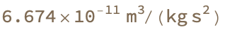
However, the current scattered information landscape of computing is marred by significant energy expenditures, an inefficiency that, theoretically, we have the means to circumvent. This principle applies to the study of quantum entanglement as well, where simulations producing diagrams with progressively sped-up loops hint at the continuous and "complex" interconnection of entangled states.
Manipulate[
 Plot[Sin[a x + b], {x, 0, 2 \[Pi]}], {a, 1, 5}, {b, 0, 2 \[Pi]}]
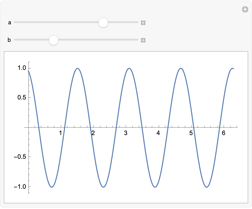
In a personal reflection, the nuances of quantum theory that was an open-close tangible experiment designed to probe the quantum realm, that was good. That has parallels with the sensory experience of food textures.
Entity["PhysicalQuantity", "Work"]["Dataset"]
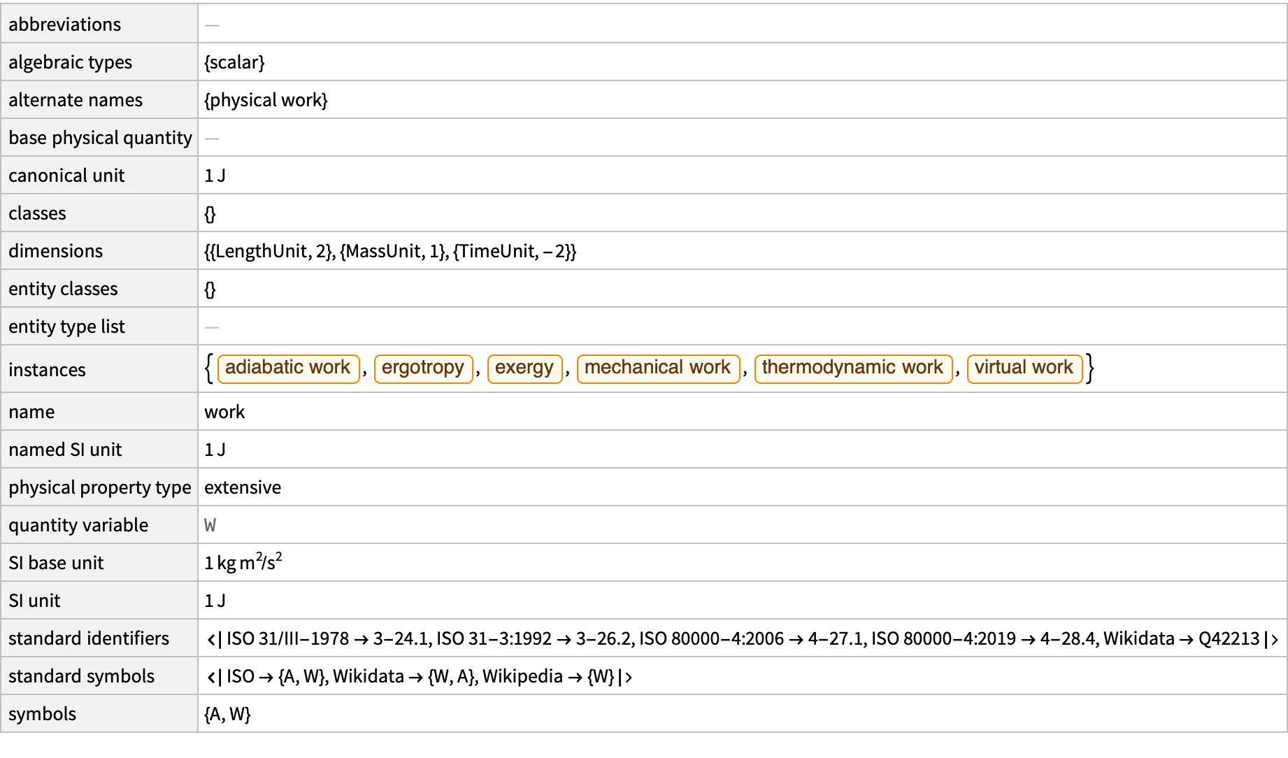
The variety in food textures, from crunchy to creamy, is directly linked to the molecular structure of proteins, illustrating a vivid connection between dietary fibers in muscle cells and other proteins. This analogy extends to digital taste, a sensory experience shaped by the molecular interaction with taste receptors and the physical composition of food as it interacts with our plate.
Table[FormulaData[formula], {formula, FormulaLookup["Work"]}]

This exploration into the "verification" of quantum entanglement is still burgeoning, akin to the creation of new sounds or musical instruments, challenging yet increasingly within our reach, including the replication of specific tastes.
FormulaData[{"Work", "Standard"}, "QuantityVariables"]
Such research holds the promise of profound implications, potentially reshaping even fields like information theory and deepening our fundamental comprehension of the cosmos.
DimensionalCombinations[{"Mass", "Distance"}, "Force",
 IncludeQuantities -> {Quantity[1, "StandardAccelerationOfGravity"]}]
It's enough to make anyone shiver, being in these cosmos. My life is officially ruined, I have been in principle knowing how to do computing in a certain way but even generating something that reminds people enough of something they knew, build that and give it to me. Give me the future, when you're buzzing around it's all very convoluted and yes, there are layers and patches. But if I'm typing in Wolfram Alpha it's like night and day I can get to that calculation in a couple of minutes. It's like doing a nuanced survey if it's the "last act" that we have with this lens of diagonal arguments, that there will be "all these" pockets of quantum irreducibility.
workFormulas = FormulaLookup["Work"]

potentialEnergyFormulas = FormulaLookup["PotentialEnergy"]

workFormula =
 FormulaData[{"Work", "Standard"}, <|
   QuantityVariable["d", "Distance"] -> Quantity[50, "Meters"],
   QuantityVariable["F", "Force"] -> Quantity[30, "Newtons"]|>]

FormulaLookup["IdealGasLaw"]


