Video Link

In a previous post I described how to geographically map the recent earthquake activity near the Bárðarbunga volcano located in the Vatnajökull National Park. This post builds on that idea to create an animation of the earthquakes over time, in this case the last 48 hours. Every frame of the animation will equate with 1 minute in real time. With a frame rate of 25 frames per second this will yield an animation lasting about 115 seconds.

We start out similarly to the previous post to get the location of the Bárðarbunga volcano and build the background image maps, which are computed once and then stored for performance reasons later on:

Bardarbunga=Entity["Volcano","Bardarbunga"];
BardarBungaCoordinates=Bardarbunga["Coordinates"];
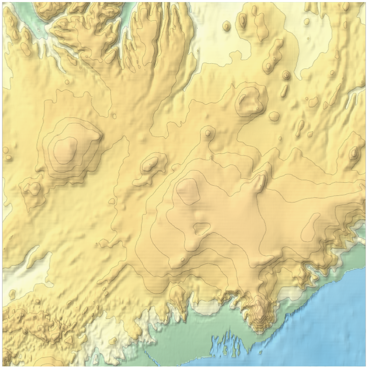
reliefmap=GeoGraphics[BardarBungaCoordinates,GeoRange->Quantity[100,"Kilometers"],GeoBackground->GeoStyling["ReliefMap"],ImageSize->{720,720}];
contourmap=GeoGraphics[BardarBungaCoordinates,GeoRange->Quantity[100,"Kilometers"],GeoBackground->GeoStyling["ContourMap"],ImageSize->{720,720}];
georange=GeoRange->(GeoRange/.Options[contourmap,GeoRange]);
baseimage=ImageCompose[reliefmap,{contourmap,.5}]

Next, we import the data and create a list with elements: {time_offset, location}

data="results"/.Import["http://apis.is/earthquake/is","JSON"];
data=Map[{"timestamp",{"latitude","longitude"}}/.#&,data];
data=Map[{DateDifference[DateObject[First[#]],DateObject[dataset2[[1,1]]],"Minute"],Last[#]}&,data];
data=Map[{QuantityMagnitude[First[#]],Last[#]}&,data];

A typical entry of data looks like {4.65, {65.057, -16.569}}, where 4.65 is the number of minutes since the first recorded earthquake data point and {65.057,-16.569} is the recorded latitude and longitude of the earthquake.

Next we define the earthquake overlay function which will superimpose all earthquakes up to minute min on the baseimage. To highlight recent earthquake the AbsolutePointSize of them is set to 10 (and older earthquakes are point size 3):

overlay[min_]:=Overlay[{
  baseimage,
  GeoGraphics[{
    Table[{Hue[0.5+c/(2min)],AbsolutePointSize[If[c>9min/10,10,3]],Point@Select[data,c-min/10<First[#]<c&][[All,2]]},{c,1,min,min/10}]
    },georange,GeoBackground->None,ImageSize->{720,720}]
  }]

Now, we will create a directory to export each movie frame (total about 3,600 frames to account for 2,880 regular frames and extra frames to allow the larger red earthquake dots to collapse into smaller 3 point dots):

basedir = "c:usersarnoudb.wribardarbunga";
If[FileType[basedir] === None, CreateDirectory[basedir]];
files = FileNames["*.png", basedir];
If[Length[files] > 0, DeleteFile[files]]

To speed up computation we will use 8 parallel kernels. I close out any old parallel kernels and then launch fresh ones:

CloseKernels[]; LaunchKernels[8];

This is the key computation which generates all the frames. It exports all 3,600 images as png files of the form geo-nnnn.png

ParallelTable[Print@Export[basedir<>"geo-"<>IntegerString[i,10,4]<>".png",overlay[i]],{i,Round[1.25(48 60)]},Method->"FinestGrained"];

The final step, generating an MP4 file, is done outside of the Wolfram Language using ffmpeg. This scans the png files and builds a mp4 video file:

C:Usersarnoudb.WRIardarbunga>c: estfmpegfmpeg.exe -i geo-%04d.png -crf 18 movie.mp4

The final result can be viewed on Vimeo.