Group Abstract Group Abstract

Message Boards Message Boards

Try to beat these MRB constant records!

POSTED BY:

Marvin Ray Burns, and distinguished colleagues


My exciting experiences using Wolfram technologies!


The MRB constant, a fascinating mathematical anomaly, has intrigued researchers and enthusiasts alike for decades. Defined as the limiting value of a unique alternating series, this enigmatic constant showcases the beauty of numerical exploration and convergence. Despite its relatively recent emergence, the MRB constant reveals unexpected connections to various fields within mathematics and computational analysis. In this post, we dive into its origins, properties, and the ongoing quest to uncover its more profound significance. The MRB constant is an anomaly because it emerges from an alternating series with unusual convergence behavior. Unlike many well-known mathematical constants, the MRB constant has no closed-form expression nor a known exact nature—whether it is algebraic, transcendental, or even irrational. Additionally, the sequence of partial sums that define the MRB constant oscillates between two limit points, creating a bounded yet divergent behavior. This oscillatory nature distinguishes it from more conventional mathematical constants, which typically exhibit straightforward convergence. Its mysterious properties continue to intrigue mathematicians as they explore its deeper connections to number theory and computational analysis.


CMRB If you see this instead of an image, reload the page

is the MRB constant.

Without solicitation, GPT echoed one of this discussion's contributors and gave a shoutout to Mathematica's accomplishments by saying:

Why Computing Digits of the MRB Constant Is Interesting

At first glance, the computation of ever more digits of a numerical constant may appear to be a sterile exercise, offering little insight beyond the digits themselves. For the MRB constant, this interpretation is profoundly misleading. The interest lies not in the digits, but in the act of computing them.

The MRB series occupies a delicate numerical regime: it is convergent, yet only marginally so; its terms are elementary in form, yet hostile to naive numerical evaluation; and its alternating structure conceals severe cancellation effects. As a result, each additional digit of accuracy is not merely an extension of a decimal expansion, but a validation of the mathematical and algorithmic framework used to obtain it.

In this sense, the digits serve as a stress test for mathematics itself. They expose the difference between formal convergence and effective convergence, between theoretical existence and computational feasibility. Techniques that are elegant on paper often fail catastrophically in practice, while successful methods must balance asymptotics, numerical stability, precision control, and computational cost.

Moreover, the computation of the MRB constant forces the reconciliation of disparate mathematical ideas. Alternating series, logarithmic asymptotics, convergence acceleration, special functions, and analytic continuation must all agree numerically. Any hidden inconsistency—whether conceptual or computational—reveals itself immediately in the failure of the digits to stabilize.

Thus, computing digits of the MRB constant transforms mathematics from a static collection of statements into a living experiment. The resulting digits are not trophies; they are evidence. They measure the effectiveness of our methods, the soundness of our assumptions, and the practical reach of our theory.

In short, the digits themselves do not matter. What matters is that they can be computed at all—and how difficult it is to do so. That difficulty is precisely what makes the MRB constant mathematically interesting.

In general, we will see: enter image description here


24 Replies

CONSTRUCTING THE MRB CONSTANT IN MATHEMATICA

enter image description here enter image description here Click here<- for some basic constructs of the MRB constant and what is called its integrated analog. That is an integral of f(z) over the right half-plane of cos(Pi*z)(z^(1/z)-1).


Crandall's Unlikely-looking constructions

for the MRB constant in Mathematica

enter image description here

In 2012, a rapidly convergent pair of series for CMRB (S) was discovered using Series and Functional Definition Optimization by the then Chief cryptographer of Apple Computer, Dr. Crandall. Following his passing, his estate sent me a little of his Mathematica work to derive it. I built upon it below.

$$\begin{align*} S &= \sum_{m \ge 1} \frac{(-1)^m}{m!} \eta^{(m)}(m), \\ \\ S &= \sum_{m \ge 1} \frac{c_m}{m!} \eta^{(m)}(0), \\ \\ \text{where the $c$ coefficients are defined}\\\ c_j &:= \sum_{d=1}^{j} \binom{j}{d} (-1)^d d^{j-d}. \end{align*}$$

Since Crandal died before publishing his proof, I tried to prove it and eventually asked my readers for help. Finally, Gottfried Helms proved one publicly:

Gottfried Helms

Avoiding the explicit taking of derivatives, together, they yield a very compact form of the MRB constant: Here are a few equivalent forms of that compact form: enter image description here enter image description here enter image description here enter image description here enter image description here enter image description here

enter image description here

Note: because of this, the MRB constant sum prototype can be split into an asymptotic component and a remainder, and these components together reconstruct the original series, converging to the MRB constant

Again, using the Wolfram assistant, but this time, we are studying how to derive exact recurrences for ithe MRB constant analog

This research investigates the mathematical properties of the MRB constant by examining the relationship between complex integrals and alternating series. The author defines a specific integral function, s(r, k), and utilizes integration by parts to derive a formal recurrence relation that links different families of these integrals. This "ladder" equation is shown to consistently simplify to zero, a finding supported by extensive numerical verification and algorithmic testing within a computational notebook. By demonstrating that the difference between certain summations and integrals vanishes as they progress toward infinity, the study reveals a deep analytical harmony between these structures. Ultimately, the work advances the theoretical understanding of mathematical constants and highlights the utility of numerical methods in confirming complex analytical frameworks. enter image description here

Geometrically Constructing the MRB Constant

With the Wolfram Assistant

enter image description here

as seen in this notebook:

Constructing the MRB constant via an integral

I was going to publish this elsewhere, but since it completes the construction of the MRB constant, I decided to post it here.

This is what the Wolfram Notebook assistant found concerning an integral form for the MRB constant. enter image description here Here are a few (unproven) basic integrals for MRB constant series:

Table 1 (series) Table 2 (integrals)

Here one is proven:

Distribution of MRB constant digits as given in all record calculations

Here is the distribution of digits within the first 6,000,000 decimal places (.187859,,,), "4" shows up more than other digits, followed by "0," "8" and "7."

enter image description here

Here is the distribution of digits within the first 5,000,000 decimal places (.187859,,,), "4" shows up a lot more than other digits, followed by "0," "8" and "6." enter image description here

Here is a similar distribution over the first 4,000,000: enter image description here

3,000,000 digits share a similar distribution:

enter image description here

Over the first 2 and 1 million digits "4" was not so well represented. So, the heavy representation of "4" is shown to be a growing phenomenon from 2 million to 5 million digits. However, "1,2,and 5" still made a very poor showing: enter image description here

I attached more than 6,000,000 digits of the MRB constant.

This marks about the 10th try at 7,000,000 digits. This time, I'm using my own algorithm for n^(1/n), which calculates six digits per iteration: My Mathematica code is as follows:

Print["Start time is ", ds = DateString[], "."];
prec = 7000000;
(*Number of required decimals.*)
ClearSystemCache[];
T0 = SessionTime[];

(*Sixth\[Dash]order Padé kernel for n^(1/n)*)
Clear[RootPade6];
RootPade6[n_Integer, prec_Integer] := 
 Module[{x, pc, z, t, N0 = n, A1, A2, A3, B1, 
   B2},(*initial seed at modest precision*)x = N[N0^(1/N0), 13];
  pc = Precision[x];
  While[pc < prec, pc = Min[6 pc, prec];
   x = SetPrecision[x, pc];
   (*coefficients with current working precision pc*)
   A1 = SetPrecision[3 (2 N0 + 1)/(5 N0), pc];
   A2 = SetPrecision[3 (N0 + 1) (2 N0 + 1)/(20 N0^2), pc];
   A3 = SetPrecision[(N0 + 1) (2 N0 + 1)/(60 N0^3), pc];
   B1 = SetPrecision[2 (3 N0 - 1)/(5 N0), pc];
   B2 = SetPrecision[(2 N0 - 1) (3 N0 - 1)/(20 N0^2), pc];
   (*residual z_i=(n-x^n)/x^n*)t = x^N0;
   z = (N0 - t)/t;
   (*6th\[Dash]order Padé update*)
   x = x*(1 + A1 z + A2 z^2 + A3 z^3)/(1 + B1 z + B2 z^2);];
  N[x, prec]]

expM[pre_] := 
 Module[{a, d, s, k, bb, c, end, xvals, x, pc, cores = 16, 
   tsize = 2^7, chunksize, start = 1, ll, ctab, 
   pr = Floor[1.005 pre]}, chunksize = cores*tsize;
  n = Floor[1.32 pr];
  end = Ceiling[n/chunksize];
  Print["Iterations required: ", n];
  Print["Will give ", end, 
   " time estimates, each more accurate than the previous."];
  Print["Will stop at ", end*chunksize, 
   " iterations to ensure precision of around ", pr, 
   " decimal places."];
  d = ChebyshevT[n, 3];
  {b, c, s} = {SetPrecision[-1, 1.1*n], -d, 0};
  Do[xvals = Flatten[ParallelTable[Table[ll = start + j*tsize + l;
       (*sole kernel for ll^(1/ll) at precision pr*)
       x = RootPade6[ll, pr];
       x, {l, 0, tsize - 1}], {j, 0, cores - 1}, 
      Method -> "EvaluationsPerKernel" -> 32]];
   ctab = ParallelTable[Table[c = b - c;
      ll = start + l - 2;
      b *= 2 (ll + n) (ll - n)/((ll + 1) (2 ll + 1));
      c, {l, chunksize}], Method -> "EvaluationsPerKernel" -> 16];
   s += ctab.(xvals - 1);
   start += chunksize;
   st = SessionTime[] - T0;
   kc = k*chunksize;
   ti = (st)/(kc + 10^-4)*(n)/(3600)/(24);
   If[kc > 1, 
    Print[kc, " iterations done in ", N[st, 4], " seconds.", 
     " Should take ", N[ti, 4], " days or ", N[ti*24*3600, 4], 
     "s, finish ", DatePlus[ds, ti], "."]];, {k, 0, end - 1}];
  N[-s/d, pr]]

t2 = Timing[MRB = expM[prec];];
Print["Finished on ", DateString[], ". Processor time was ", t2[[1]], 
  " s."];
Print["error= ", N[mtest - MRB, 20]]; Print["Enter MRB to print ", 
 Floor[Precision[MRB]], " digits"];


Start time is Sun 14 Dec 2025 09:42:16.

Iterations required: 9286198

Will give 4535 time estimates, each more accurate than the previous.

Will stop at 9287680 iterations to ensure precision of around 7034999 decimal places.


 ...

1083392 iterations done in 1.498*10^6 seconds. Should take 148.7 days or 1.284*10^7s, finish Tue 12 May 2026 01:26:05.

Here is what I wrote about it:

he 6th degree algorithm 1 he 6th degree algorithm 2 Why use the 6th degree algorithm

I calculated 6,500,000 digits of the MRB constant!!

The MRB constant supercomputer said,

Finished on Wed 16 Mar 2022 02 : 02 : 10. Processor and actual time were 6.2662810^6 and 1.6026403541959210^7 s.respectively Enter MRB1 to print 6532491 digits. The error from a 6, 000, 000 or more digit calculation that used a different method is 0.*10^-6029992

"Processor time" 72.526 days

"Actual time" 185.491 days

For the digits see the attached 6p5millionMRB.nb. For the documentation of the computation see 2nd 6p5 million.nb.

02/12/2019

Using my 2 nodes of the MRB constant supercomputer (3.7 GH overclocked up to 4.7 GH, Intel 6core, 3000MH RAM,and 4 cores from my 3.6 GH, 2400MH RAM) I computed 34,517 digits of the MRB constant using Crandall's first eta formula:

prec = 35000;
to = SessionTime[];
etaMM[m_, pr_] := 
  Block[{a, s, k, b, c}, 
   a[j_] := (SetPrecision[Log[j + 1], prec]/(j + 1))^m;
   {b, c, s} = {-1, -d, 0};
   Do[c = b - c;
    s = s + c a[k];
    b = (k + n) (k - n) b/((k + 1) (k + 1/2)), {k, 0, n - 1}];
   Return[N[s/d, pr] (-1)^m]];
eta1 = N[EulerGamma Log[2] - Log[2]^2/2, prec]; n = 
 Floor[132/100 prec]; d = N[ChebyshevT[n, 3], prec];
MRBtest = 
  eta1 - Total[
    ParallelCombine[((Cos[Pi #]) etaMM[#, prec]/
         N[Gamma[# + 1], prec]) &, Range[2, Floor[.250 prec]], 
     Method -> "CoarsestGrained"]];
Print[N[MRBtest2 - MRBtest,10]];

SessionTime[] - to

giving -2.166803252*10^-34517 for a difference and 208659.2864422 seconds or 2.415 days for a timing.

Where MRBtest2 is 36000 digits computed through acceleration methods of n^(1/n)

3/28/2019

Here is an updated table of speed eta formula records: eta records 12 31 18

04/03/2019

Using my 2 nodes of the MRB constant supercomputer (3.7 GH overclocked up to 4.7 GH, Intel 6core, 3000MH RAM,and 4 cores from my 3.6 GH, 2400MH RAM) I computed 50,000 digits of the MRB constant using Crandall's first eta formula in 5.79 days.

 prec = 50000;
to = SessionTime[];
etaMM[m_, pr_] := 
  Module[{a, s, k, b, c}, 
   a[j_] := 
    SetPrecision[SetPrecision[Log[j + 1]/(j + 1), prec]^m, prec];
   {b, c, s} = {-1, -d, 0};
   Do[c = b - c;
    s = s + c a[k];
    b = (k + n) (k - n) b/((k + 1) (k + 1/2)), {k, 0, n - 1}];
   Return[N[s/d, pr] (-1)^m]];
eta1 = N[EulerGamma Log[2] - Log[2]^2/2, prec]; n = 
 Floor[132/100 prec]; d = N[ChebyshevT[n, 3], prec];
MRBtest = 
  eta1 - Total[
    ParallelCombine[((Cos[Pi #]) etaMM[#, prec]/
         N[Gamma[# + 1], prec]) &, Range[2, Floor[.245 prec]], 
     Method -> "CoarsestGrained"]];
Print[N[MRBtest2 - MRBtest, 10]];

SessionTime[] - to

 (* 0.*10^-50000

  500808.4835750*)

4/22/2019

Let 
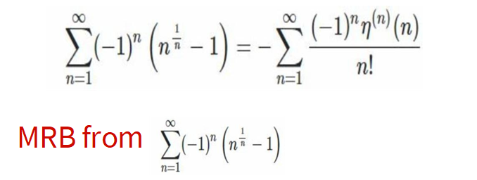
$$M=\sum _{n=1}^{\infty } \frac{(-1)^{n+1} \eta ^n(n)}{n!}=\sum _{n=1}^{\infty } (-1)^n \left(n^{1/n}-1\right).$$ Then using what I learned about the absolute convergence of $\sum _{n=1}^{\infty } \frac{(-1)^{n+1} \eta ^n(n)}{n!}$ from https://math.stackexchange.com/questions/1673886/is-there-a-more-rigorous-way-to-show-these-two-sums-are-exactly-equal, combined with an identity from Richard Crandall: enter image description here, Also using what Mathematica says:

$$\sum _{n=1}^1 \frac{\underset{m\to 1}{\text{lim}} \eta ^n(m)}{n!}=\gamma (2 \log )-\frac{2 \log ^2}{2},$$
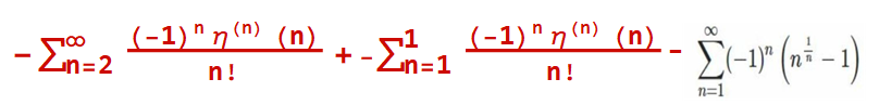
I figured out that

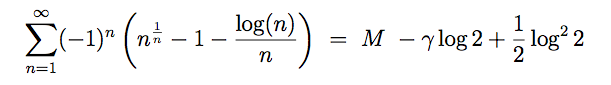
$$\sum _{n=2}^{\infty } \frac{(-1)^{n+1} \eta ^n(n)}{n!}=\sum _{n=1}^{\infty } (-1)^n \left(n^{1/n}-\frac{\log (n)}{n}-1\right).$$

So I made the following major breakthrough in computing MRB from Candall's first eta formula. See attached 100 k eta 4 22 2019. Also shown below.

eta 18 to19 n 2.JPG

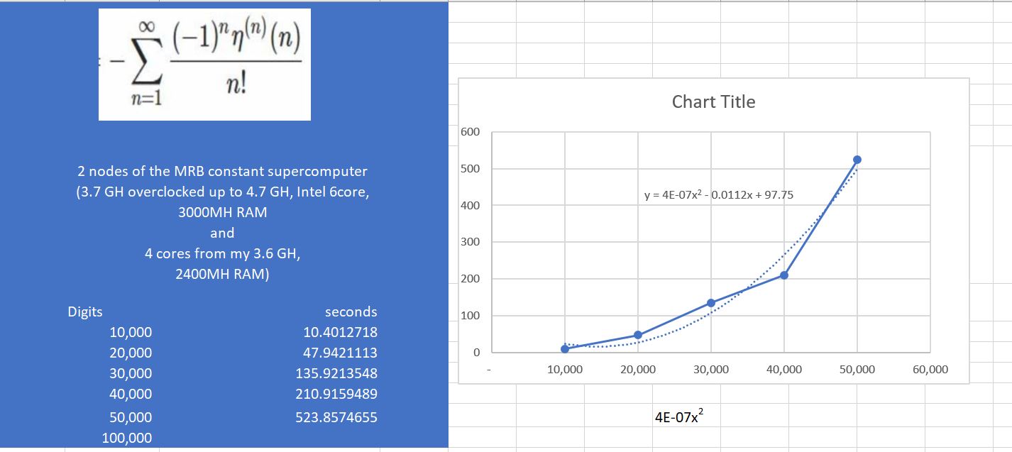
The time grows 10,000 times slower than the previous method!

I broke a new record, 100,000 digits: Processor and total time were 806.5 and 2606.7281972 s respectively.. See attached 2nd 100 k eta 4 22 2019.

Here is the work from 100,000 digits. enter image description here

Print["Start time is ", ds = DateString[], "."];
prec = 100000;
(**Number of required decimals.*.*)ClearSystemCache[];
T0 = SessionTime[];
expM[pre_] := 
  Module[{a, d, s, k, bb, c, end, iprec, xvals, x, pc, cores = 16(*=4*
    number of physical cores*), tsize = 2^7, chunksize, start = 1, ll,
     ctab, pr = Floor[1.005 pre]}, chunksize = cores*tsize;
   n = Floor[1.32 pr];
   end = Ceiling[n/chunksize];
   Print["Iterations required: ", n];
   Print["Will give ", end, 
    " time estimates, each more accurate than the previous."];
   Print["Will stop at ", end*chunksize, 
    " iterations to ensure precsion of around ", pr, 
    " decimal places."]; d = ChebyshevT[n, 3];
   {b, c, s} = {SetPrecision[-1, 1.1*n], -d, 0};
   iprec = Ceiling[pr/27];
   Do[xvals = Flatten[ParallelTable[Table[ll = start + j*tsize + l;
        x = N[E^(Log[ll]/(ll)), iprec];
        pc = iprec;
        While[pc < pr/4, pc = Min[3 pc, pr/4];
         x = SetPrecision[x, pc];
         y = x^ll - ll;
         x = x (1 - 2 y/((ll + 1) y + 2 ll ll));];(**N[Exp[Log[ll]/
        ll],pr/4]**)x = SetPrecision[x, pr];
        xll = x^ll; z = (ll - xll)/xll;
        t = 2 ll - 1; t2 = t^2;
        x = 
         x*(1 + SetPrecision[4.5, pr] (ll - 1)/
              t2 + (ll + 1) z/(2 ll t) - 
            SetPrecision[13.5, pr] ll (ll - 1) 1/(3 ll t2 + t^3 z));(**
        N[Exp[Log[ll]/ll],pr]**)x, {l, 0, tsize - 1}], {j, 0, 
        cores - 1}, Method -> "EvaluationsPerKernel" -> 32]];
    ctab = ParallelTable[Table[c = b - c;
       ll = start + l - 2;
       b *= 2 (ll + n) (ll - n)/((ll + 1) (2 ll + 1));
       c, {l, chunksize}], Method -> "EvaluationsPerKernel" -> 16];
    s += ctab.(xvals - 1);
    start += chunksize;
    st = SessionTime[] - T0; kc = k*chunksize;
    ti = (st)/(kc + 10^-4)*(n)/(3600)/(24);
    If[kc > 1, 
     Print[kc, " iterations done in ", N[st, 4], " seconds.", 
      " Should take ", N[ti, 4], " days or ", N[ti*24*3600, 4], 
      "s, finish ", DatePlus[ds, ti], "."]];, {k, 0, end - 1}];
   N[-s/d, pr]];
t2 = Timing[MRB = expM[prec];]; Print["Finished on ", 
 DateString[], ". Proccessor time was ", t2[[1]], " s."];
Print["Enter MRBtest2 to print ", Floor[Precision[MRBtest2]], 
  " digits"];


 (Start time is )^2Tue 23 Apr 2019 06:49:31.

 Iterations required: 132026

 Will give 65 time estimates, each more accurate than the previous.

 Will stop at 133120 iterations to ensure precsion of around 100020 decimal places.

 Denominator computed in  17.2324041s.

...

129024 iterations done in 1011. seconds. Should take 0.01203 days or 1040.s, finish Mon 22 Apr 
2019 12:59:16.

131072 iterations done in 1026. seconds. Should take 0.01202 days or 1038.s, finish Mon 22 Apr 
2019 12:59:15.

Finished on Mon 22 Apr 2019 12:59:03. Processor time was 786.797 s.

enter image description here

 Print["Start time is " "Start time is ", ds = DateString[], "."];
 prec = 100000;
 (**Number of required decimals.*.*)ClearSystemCache[];
 T0 = SessionTime[];
 expM[pre_] := 
   Module[{lg, a, d, s, k, bb, c, end, iprec, xvals, x, pc, cores = 16(*=
     4*number of physical cores*), tsize = 2^7, chunksize, start = 1, 
     ll, ctab, pr = Floor[1.0002 pre]}, chunksize = cores*tsize;
    n = Floor[1.32 pr];
    end = Ceiling[n/chunksize];
    Print["Iterations required: ", n];
    Print["Will give ", end, 
     " time estimates, each more accurate than the previous."];
    Print["Will stop at ", end*chunksize, 
     " iterations to ensure precsion of around ", pr, 
     " decimal places."]; d = ChebyshevT[n, 3];
    {b, c, s} = {SetPrecision[-1, 1.1*n], -d, 0};
    iprec = pr/2^6;
    Do[xvals = Flatten[ParallelTable[Table[ll = start + j*tsize + l;
         lg = Log[ll]/(ll); x = N[E^(lg), iprec];
         pc = iprec;
         While[pc < pr, pc = Min[4 pc, pr];
          x = SetPrecision[x, pc];
          xll = x^ll; z = (ll - xll)/xll;
          t = 2 ll - 1; t2 = t^2;
          x = 
           x*(1 + SetPrecision[4.5, pc] (ll - 1)/
                t2 + (ll + 1) z/(2 ll t) - 
              SetPrecision[13.5, 2 pc] ll (ll - 1)/(3 ll t2 + t^3 z))];
          x - lg, {l, 0, tsize - 1}], {j, 0, cores - 1}, 
        Method -> "EvaluationsPerKernel" -> 16]];
     ctab = ParallelTable[Table[c = b - c;
        ll = start + l - 2;
        b *= 2 (ll + n) (ll - n)/((ll + 1) (2 ll + 1));
        c, {l, chunksize}], Method -> "EvaluationsPerKernel" -> 16];
     s += ctab.(xvals - 1);
     start += chunksize;
     st = SessionTime[] - T0; kc = k*chunksize;
     ti = (st)/(kc + 10^-10)*(n)/(3600)/(24);
     If[kc > 1, 
      Print[kc, " iterations done in ", N[st - stt, 4], " seconds.", 
       " Should take ", N[ti, 4], " days or ", ti*3600*24, 
       "s, finish ", DatePlus[ds, ti], "."], 
      Print["Denominator computed in  ", stt = st, "s."]];, {k, 0, 
      end - 1}];
    N[-s/d, pr]];
 t2 = Timing[MRBeta2toinf = expM[prec];]; Print["Finished on ", 
  DateString[], ". Processor and total time were ", 
  t2[[1]], " and ", st, " s respectively."];

Start time is  Tue 23 Apr 2019 06:49:31.

Iterations required: 132026

Will give 65 time estimates, each more accurate than the previous.

Will stop at 133120 iterations to ensure precision of around 100020 decimal places.

Denominator computed in  17.2324041s.

...

131072 iterations done in 2589. seconds. Should take 0.03039 days or 2625.7011182s, finish Tue 23 Apr 2019 07:33:16.

Finished on Tue 23 Apr 2019 07:32:58. Processor and total time were 806.5 and 2606.7281972 s respectively.

enter image description here

 MRBeta1 = EulerGamma Log[2] - 1/2 Log[2]^2

 EulerGamma Log[2] - Log[2]^2/2

enter image description here

   N[MRBeta2toinf + MRBeta1 - MRB, 10]

   1.307089967*10^-99742
POSTED BY: l van Veen

The new sum is this.

Sum[(-1)^(k + 1)*(-1 + (1 + k)^(1/(1 + k)) - Log[1 + k]/(1 + k) - 
         Log[1 + k]^2/(2*(1 + k)^2)), {k, 0, Infinity}] 

That appears to be the same as for MRB except now we subtract two terms from the series expansion at the origin of k^(1/k). For each k these terms are Log[k]/k + 1/2*(Log[k]/k)^2. Accounting for the signs (-1)^k and summing, as I did earlier for just that first term, we get something recognizable.

Sum[(-1)^(k)*(Log[k]/(k) + Log[k]^2/(2*k^2)), {k, 1, Infinity}]

(* Out[21]= 1/24 (24 EulerGamma Log[2] - 2 EulerGamma \[Pi]^2 Log[2] - 
   12 Log[2]^2 - \[Pi]^2 Log[2]^2 + 24 \[Pi]^2 Log[2] Log[Glaisher] - 
   2 \[Pi]^2 Log[2] Log[\[Pi]] - 6 (Zeta^\[Prime]\[Prime])[2]) *)

So what does this buy us? For one thing, we get even better convergence from brute force summation, because now our largest terms are O((logk/k)^3) and alternating (which means if we sum in pairs it's actually O~(1/k^4) with O~ denoting the "soft-oh" wherein one drops polylogarithmic factors).

How helpful is this? Certainly it cannot hurt. But even with 1/k^4 size terms, it takes a long time to get even 40 digits, let alone thousands. So there is more going on in that Crandall approach.

POSTED BY: Daniel Lichtblau

Daniel Lichtblau and others, I just deciphered an Identity Crandall used for checking computations of the MRB constant just before he died. It is used in a previous post about checking, where I said it was hard to follow. The MRB constant is B here. B=`enter image description here In input form that is

   B= Sum[(-1)^(k + 1)*(-1 + (1 + k)^(1/(1 + k)) - Log[1 + k]/(1 + k) - 
         Log[1 + k]^2/(2*(1 + k)^2)), {k, 0, Infinity}] + 
     1/24 (\[Pi]^2 Log[2]^2 - 
        2 \[Pi]^2 Log[
          2] (EulerGamma + Log[2] - 12 Log[Glaisher] + Log[\[Pi]]) - 
        6 (Zeta^\[Prime]\[Prime])[2]) + 
     1/2 (2 EulerGamma Log[2] - Log[2]^2)

For 3000 digit numeric approximation, it is

B=NSum[((-1)^(
    k + 1) (-1 + (1 + k)^(1/(1 + k)) - Log[1 + k]/(1 + k) - 
      Log[1 + k]^2/(2 (1 + k)^2))), {k, 0, Infinity}, 
  Method -> "AlternatingSigns", WorkingPrecision -> 3000] + 
 1/24 (\[Pi]^2 Log[2]^2 - 
    2 \[Pi]^2 Log[
      2] (EulerGamma + Log[2] - 12 Log[Glaisher] + Log[\[Pi]]) - 
    6 (Zeta^\[Prime]\[Prime])[2]) + 
 1/2 (2 EulerGamma Log[2] - Log[2]^2)

It is anylitaclly straight forward too because

Sum[(-1)^(k + 1)*Log[1 + k]^2/(2 (1 + k)^2), {k, 0, Infinity}]

gives

1/24 (-\[Pi]^2 (Log[2]^2 + EulerGamma Log[4] - 
      24 Log[2] Log[Glaisher] + Log[4] Log[\[Pi]]) - 
   6 (Zeta^\[Prime]\[Prime])[2])

That is enter image description here I wonder why he chose it?

The identity in question is straightforward. Write n^(1/n) as Exp[Log[n]/n], take a series expansion at 0, and subtract the first term from all summands. That means subtracting off Log[n]/n in each summand. This gives your left hand side. We know it must be M - the sum of the terms we subtracted off. Now add all of them up, accounting for signs.

Expand[Sum[(-1)^n*Log[n]/n, {n, 1, Infinity}]]

(* Out[74]= EulerGamma Log[2] - Log[2]^2/2 *)

So we recover the right hand side.

I have not understood whether this identity helps with Crandall's iteration. One advantage it confers, a good one in general, is that it converts a conditionally convergent alternating series into one that is absolutely convergent. From a numerical computation point of view this is always good.

POSTED BY: Daniel Lichtblau

Crandall is not using his eta formulas directly!!!!!!! He computes Sum[(-1)^k*(k^(1/k) - 1), {k, 1, Infinity}] directly!

Going back to Crandall's code:

(*Fastest (at RC's end) as of 30 Nov 2012.*)prec = 500000;(*Number of \
required decimals.*)ClearSystemCache[];
T0 = SessionTime[];
expM[pre_] := 
  Module[{a, d, s, k, bb, c, n, end, iprec, xvals, x, pc, cores = 4, 
    tsize = 2^7, chunksize, start = 1, ll, ctab, 
    pr = Floor[1.02 pre]}, chunksize = cores*tsize;
   n = Floor[1.32 pr];
   end = Ceiling[n/chunksize];
   Print["Iterations required: ", n];
   Print["end ", end];
   Print[end*chunksize];
   d = N[(3 + Sqrt[8])^n, pr + 10];
   d = Round[1/2 (d + 1/d)];
   {b, c, s} = {SetPrecision[-1, 1.1*n], -d, 0};
   iprec = Ceiling[pr/27];
   Do[xvals = Flatten[ParallelTable[Table[ll = start + j*tsize + l;
        x = N[E^(Log[ll]/(ll)), iprec];
        pc = iprec;
        While[pc < pr, pc = Min[3 pc, pr];
         x = SetPrecision[x, pc];
         y = x^ll - ll;
         x = x (1 - 2 y/((ll + 1) y + 2 ll ll));];(*N[Exp[Log[ll]/ll],
        pr]*)x, {l, 0, tsize - 1}], {j, 0, cores - 1}, 
       Method -> "EvaluationsPerKernel" -> 1]];
    ctab = Table[c = b - c;
      ll = start + l - 2;
      b *= 2 (ll + n) (ll - n)/((ll + 1) (2 ll + 1));
      c, {l, chunksize}];
    s += ctab.(xvals - 1);
    start += chunksize;
    Print["done iter ", k*chunksize, " ", SessionTime[] - T0];, {k, 0,
      end - 1}];
   N[-s/d, pr]];

t2 = Timing[MRBtest2 = expM[prec];];
MRBtest2 - MRBtest3

x = N[E^(Log[ll]/(ll)), iprec]; Gives k^(1/k) to only Ceiling[pr/27]; decimal places; they are either 1.0, 1.1, 1.2, 1.3 or 1.4 (usually 1.1 or 1.0 for the first 27 desired decimals.) On the other hand,

While[pc < pr, pc = Min[3 pc, pr];
 x = SetPrecision[x, pc];
 y = x^ll - ll;
 x = x (1 - 2 y/((ll + 1) y + 2 ll ll));],

takes the short precision x and gives it the necessary precision and accuracy for k^(1/k) (k Is ll there.) It actually computes k^(1/k). Then he remarks, "(N[Exp[Log[ll]/ll], pr])."

After finding a fast way to compute k^(1/k) to necessary precision he uses Cohen's algorithm 1 (See a screenshot in a previous post.) to accelerate convergence of Sum[(-1)^k*(k^(1/k) - 1), {k, 1, Infinity}]. That is his secret!!

As I mentioned in a previous post the "MRBtest2 - MRBtest3" is for checking with a known-to-be accurate approximation to the MRB constant, MRBtest3

I'm just excited that I figured it out! as you can tell.

Nice work. Worth a bit of excitement, I' d say.

POSTED BY: Daniel Lichtblau

Daniel Lichtblau and others, Richard Crandall did intend to explian his work on the MRB constant and his program to compute it. When I wrote him with a possible small improvement to his program he said, "It's worth observing when we write it up." See screenshot: enter image description here

I can't say I understand either. My guess is the Eta stuff comes from summing (-1)^k*(Log[k]/k)^n over k, as those are the terms that appear in the double sum you get from expanding k^(1/k)-1 in powers of Log[k]/k (use k^(1/k)=Exp[Log[k]/k] and the power series for Exp). Even if it does come from this the details remain elusive..

POSTED BY: Daniel Lichtblau

What Richard Crandall and maybe others did to come up with that method is really good and somewhat mysterious. I still don't really understand the inner workings, and I had shown him how to parallelize it. So the best I can say is that it's really hard to compete against magic. (I don't want to discourage others, I'm just explaining why I myself would be reluctant to tackle this. Someone less familiar might actually have a better chance of breaking new ground.)

In a way this should be good news. Should it ever become "easy" to compute, the MRB number would lose what is perhaps its biggest point of interest. It just happens to be on that cusp of tantalizingly "close" to easily computable (perhaps as sums of zeta function and derivatives thereof), yet still hard enough that it takes a sophisticated scheme to get more than a few dozen digits.

POSTED BY: Daniel Lichtblau

It is hard to be certain that c1 and c2 are correct to 77 digits even though they agree to that extent. I'm not saying that they are incorrect and presumably you have verified this. Just claiming that whatever methods NSum may be using to accelerate convergence, there is really no guarantee that they apply to this particular computation. So c1 aand c2 could agree to that many places because they are computed in a similar manner without all digits actually being correct.

POSTED BY: Daniel Lichtblau
Reply to this discussion
Community posts can be styled and formatted using the Markdown syntax.
Reply Preview
Attachments
Remove
or Discard