If above this you see the title "Try to beat these MRB constant records!" in order to see the first 11 sections, you'll need to refresh the page.
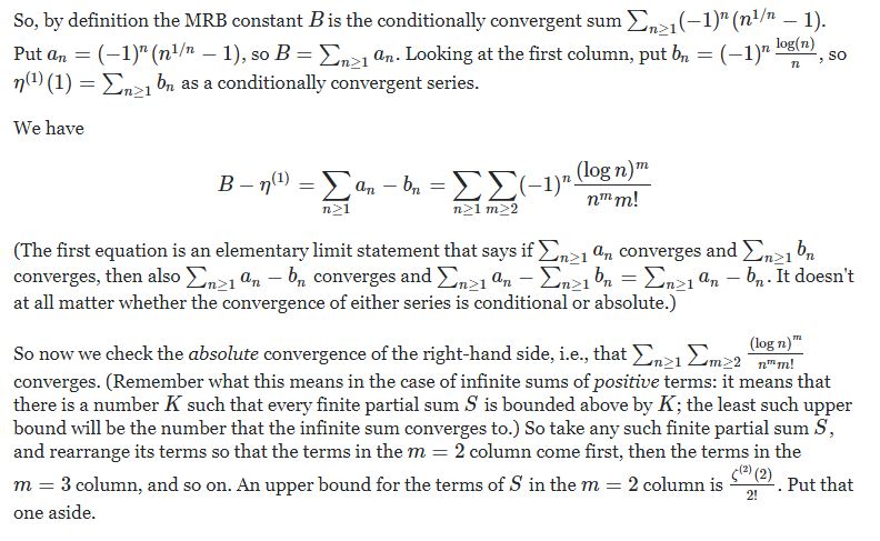
MRB constant formulas and identities
I developed this informal catalog of formulas for the MRB constant with over 20 years of research and ideas from users like you.
6/7/2022
CMRB
=
=
=
=
=
=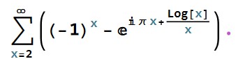
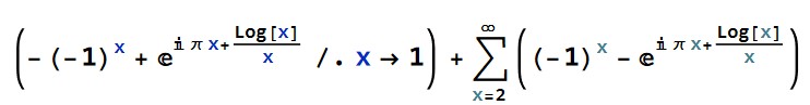
So, using induction, we have.
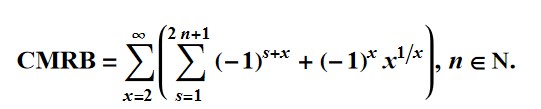
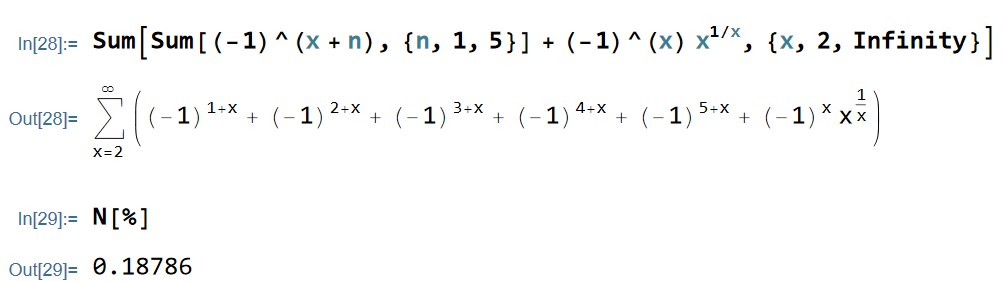
Sum[Sum[(-1)^(x + n), {n, 1, 5}] + (-1)^(x) x^(1/x), {x, 2, Infinity}]
3/25/2022
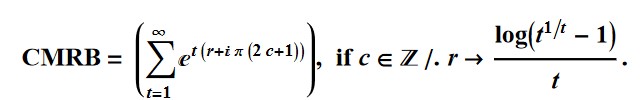
Formula (11) =
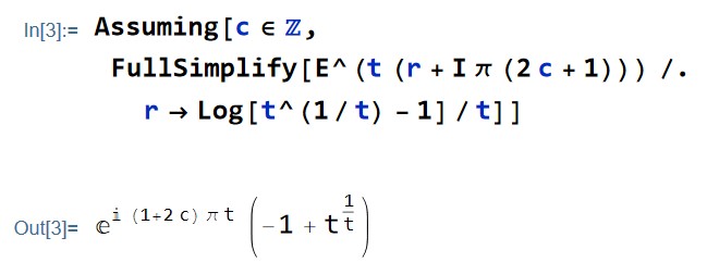
As Matheamatica says:
Assuming[Element[c, \[DoubleStruckCapitalZ]], FullSimplify[
     E^(t*(r + I*Pi*(2*c + 1))) /. r -> Log[t^(1/t) - 1]/t]]
= E^(I (1 + 2 c) [Pi] t) (-1 + t^(1/t))
Where for all integers c, (1+2c) is odd leading to 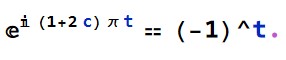
Expanding the E^log term gives
which is 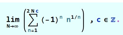 ,
,
That is exactly (2) in the above-quoted MathWorld definition:

2/21/2022
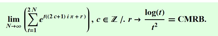
Directly from the formula of 12/29/2021 below,
 In
In
u = (-1)^t; N[
NSum[(t^(1/t) - 1) u, {t, 1, Infinity }, WorkingPrecision -> 24,
Method -> "AlternatingSigns"], 15]
Out[276]= 0.187859642462067
In
v = (-1)^-t - (-1)^t; 2 I N[
NIntegrate[Im[(t^(1/t) - 1) v^-1], {t, 1, Infinity I},
WorkingPrecision -> 24], 15]
Out[278]= 0.187859642462067
Likewise,
Expanding the exponents,
 This can be generalized to
Building upon that, we get a closed form for the inner integral in the following.
CMRB=
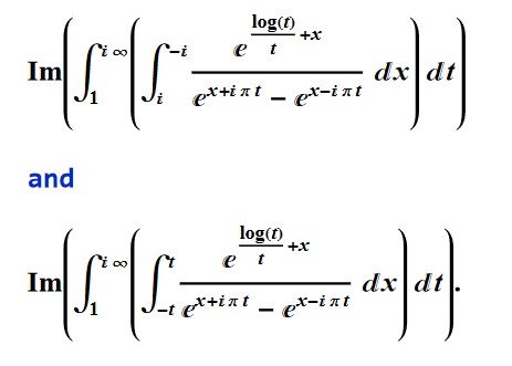
In[1]:=
CMRB = NSum[(-1)^n (n^(1/n) - 1), {n, 1, Infinity},
   WorkingPrecision -> 1000, Method -> "AlternatingSigns"];

In[2]:= CMRB - {
 Quiet[Im[NIntegrate[
    Integrate[
     E^(Log[t]/t + x)/(-E^((-I)*Pi*t + x) + E^(I*Pi*t + x)), {x,
      I, -I}], {t, 1, Infinity I}, WorkingPrecision -> 200,
    Method -> "Trapezoidal"]]];
 Quiet[Im[NIntegrate[
    Integrate[
     Im[E^(Log[t]/t + x)/(-E^((-I)*Pi*t + x) + E^(I*Pi*t + x))], {x,
      -t,  t }], {t, 1
     , Infinity  I}, WorkingPrecision -> 2000,
    Method -> "Trapezoidal"]]]}

Out[2]= {3.*10^-998, 3.*10^-998}
Which after a little analysis, can be shown convergent in the continuum limit at t → ∞ i.
12/29/2021
From "Primary Proof 1" worked below, it can be shown that
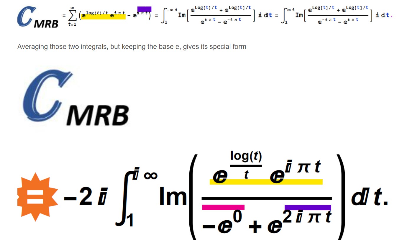
Mathematica knows that because
  m = N[NSum[-E^(I*Pi*t) + E^(I*Pi*t)*t^t^(-1), {t, 1, Infinity},
      Method -> "AlternatingSigns", WorkingPrecision -> 27], 18];
  Print[{m -
     N[NIntegrate[
       Im[(E^(Log[t]/t) + E^(Log[t]/t))/(E^(I \[Pi] t) -
            E^(-I \[Pi] t))] I, {t, 1, -Infinity I},
       WorkingPrecision -> 20], 18],
    m - N[NIntegrate[
       Im[(E^(Log[t]/t) + E^(Log[t]/t))/(E^(-I \[Pi] t) -
            E^(I \[Pi] t))] I, {t, 1, Infinity I},
       WorkingPrecision -> 20], 18],
    m + 2 I*NIntegrate[
       Im[(E^(I*Pi*t + Log[t]/t))/(-1 + E^((2*I)*Pi*t))], {t, 1,
        Infinity I}, WorkingPrecision -> 20]}]
yields
{0.*^-19,0.*^-19,0.*^-19}
Partial sums to an upper limit of (10^n i) give approximations for the MRB constant + the same approximation *10^-(n+1) i.
Example:
-2 I*NIntegrate[
  Im[(E^(I*Pi*t + Log[t]/t))/(-1 + E^((2*I)*Pi*t))], {t, 1, 10^7 I},
  WorkingPrecision -> 20]
gives
0.18785602000738908694 + 1.878560200074*10^-8 I
where CMRB ≈ 0.187856.
Notice it is special because if we integrate only the numerator, we have MKB=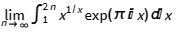 , which defines the "integrated analog of CMRB" (MKB) described by Richard Mathar in https://arxiv.org/abs/0912.3844. (He called it M1.)
Like how this:
NIntegrate[(E^(I*Pi*t + Log[t]/t)), {t, 1, Infinity I},
  WorkingPrecision -> 20] - I/Pi
converges to
0.070776039311528802981 - 0.68400038943793212890 I.
(The upper limits " i infinity" and " infinity" produce the same result in this integral.)
11/14/2021
Here is a standard notation for the above mentioned
CMRB,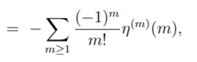
 .
.
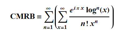
In[16]:= CMRB = 0.18785964246206712024851793405427323005590332204; \
CMRB - NSum[(Sum[
    E^(I \[Pi] x) Log[x]^n/(n! x^n), {x, 1, Infinity}]), {n, 1, 20},
  WorkingPrecision -> 50]

Out[16]= -5.8542798212228838*10^-30

In[8]:= c1 =
 Activate[Limit[(-1)^m/m! Derivative[m][DirichletEta][x] /. m -> 1,
   x -> 1]]

Out[8]= 1/2 Log[2] (-2 EulerGamma + Log[2])

In[14]:= CMRB -
 N[-(c1 + Sum[(-1)^m/m! Derivative[m][DirichletEta][m], {m, 2, 20}]),
  30]

Out[14]= -6.*10^-30
11/01/2021
: The catalog now appears complete, and can all be proven through Primary Proof 1, and the one with the eta function, Primary Proof 2, both found below.
a ≠b
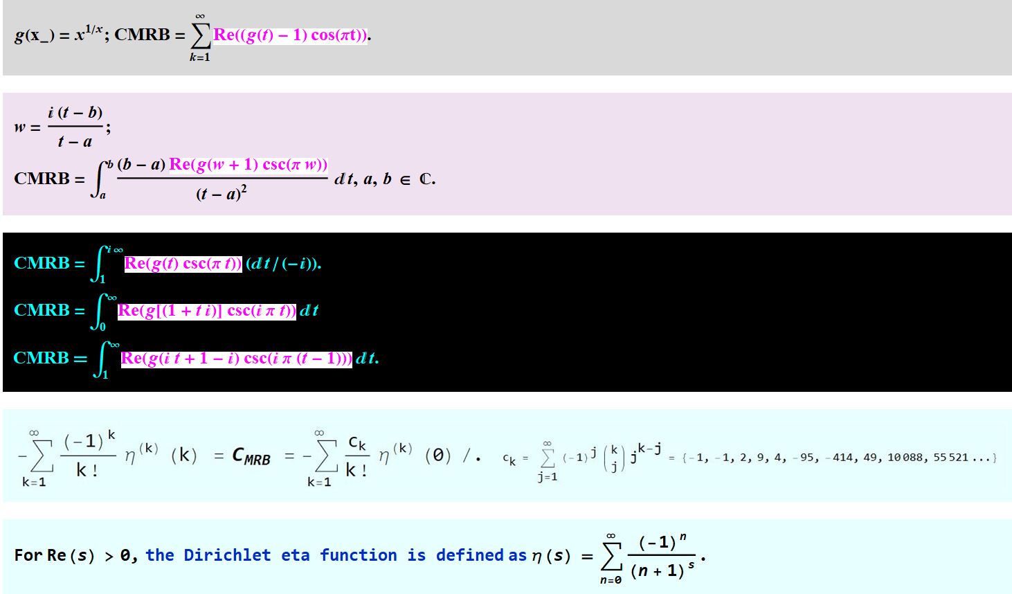
g[x_] = x^(1/x); CMRB =
 NSum[(-1)^k (g[k] - 1), {k, 1, Infinity}, WorkingPrecision -> 100,
  Method -> "AlternatingSigns"]; a = -Infinity I; b = Infinity I;
g[x_] = x^(1/x); (v = t/(1 + t + t I);
 Print[CMRB - (-I /2 NIntegrate[ Re[v^-v Csc[Pi/v]]/ (t^2), {t, a, b},
       WorkingPrecision -> 100])]); Clear[a, b]
    -9.3472*10^-94
Thus, we find
here, and
 next:
next:
In[93]:= CMRB =
 NSum[Cos[Pi n] (n^(1/n) - 1), {n, 1, Infinity},
  Method -> "AlternatingSigns", WorkingPrecision -> 100]; Table[
 CMRB - (1/2 +
    NIntegrate[
     Im[(t^(1/t) - t^(2 n))] (-Csc[\[Pi] t]), {t, 1, Infinity I},
     WorkingPrecision -> 100, Method -> "Trapezoidal"]), {n, 1, 5}]

Out[93]= {-9.3472*10^-94, -9.3473*10^-94, -9.3474*10^-94, \
-9.3476*10^-94, -9.3477*10^-94}
CNT+F "The following is a way to compute the" for more evidence
For such n, 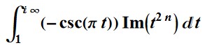 converges to 1/2+0i.
(How I came across all of those and more example code follow in various replies.)
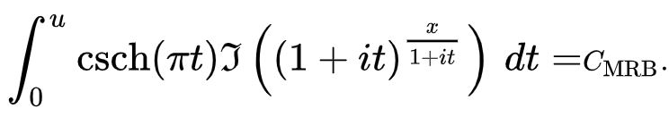
On 10/18/2021
, I found the following triad of pairs of integrals summed from -complex infinity to +complex infinity.
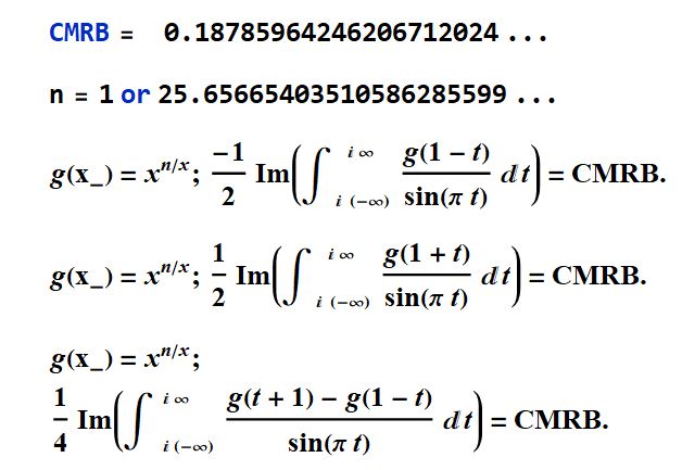
You can see it worked in this link here.
In[1]:= n = {1, 25.6566540351058628559907};

In[2]:= g[x_] = x^(n/x);
-1/2 Im[N[
   NIntegrate[(g[(1 - t)])/(Sin[\[Pi] t]), {t, -Infinity I,
     Infinity I}, WorkingPrecision -> 60], 20]]

Out[3]= {0.18785964246206712025, 0.18785964246206712025}

In[4]:= g[x_] = x^(n/x);
1/2 Im[N[NIntegrate[(g[(1 + t)])/(Sin[\[Pi] t]), {t, -Infinity I,
     Infinity I}, WorkingPrecision -> 60], 20]]

Out[5]= {0.18785964246206712025, 0.18785964246206712025}

In[6]:= g[x_] = x^(n/x);
1/4 Im[N[NIntegrate[(g[(1 + t)] - (g[(1 - t)]))/(Sin[\[Pi] t]), {t, -Infinity I,
     Infinity I}, WorkingPrecision -> 60], 20]]

Out[7]= {0.18785964246206712025, 0.18785964246206712025}
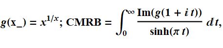
Therefore, bringing
back to mind, we joyfully find,
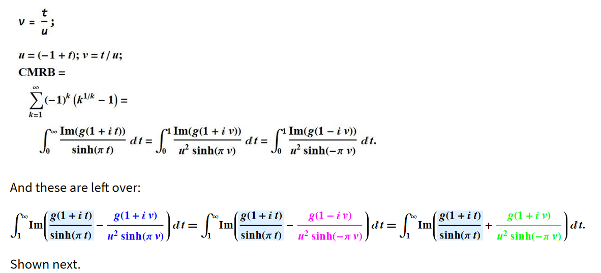
In[1]:= n =
  25.65665403510586285599072933607445153794770546058072048626118194900\
97321718621288009944007124739159792146480733342667`100.;

g[x_] = {x^(1/x), x^(n/x)};

CMRB = NSum[(-1)^k (k^(1/k) - 1), {k, 1, Infinity},
   WorkingPrecision -> 100, Method -> "AlternatingSigns"];

Print[CMRB -
  NIntegrate[Im[g[(1 + I t)]/Sinh[\[Pi] t]], {t, 0, Infinity},
   WorkingPrecision -> 100], u = (-1 + t); v = t/u;
 CMRB - NIntegrate[Im[g[(1 + I v)]/(Sinh[\[Pi] v] u^2)], {t, 0, 1},
   WorkingPrecision -> 100],
 CMRB - NIntegrate[Im[g[(1 - I v)]/(Sinh[-\[Pi] v] u^2)], {t, 0, 1},
   WorkingPrecision -> 100]]

During evaluation of In[1]:= {-9.3472*10^-94,-9.3472*10^-94}{-9.3472*10^-94,-9.3472*10^-94}{-9.3472*10^-94,-9.3472*10^-94}

In[23]:= Quiet[
 NIntegrate[
  Im[g[(1 + I t)]/Sinh[\[Pi] t] -
    g[(1 + I v)]/(Sinh[\[Pi] v] u^2)], {t, 1, Infinity},
  WorkingPrecision -> 100]]

Out[23]= -3.\
9317890831820506378791034479406121284684487483182042179057328100219696\
20202464096600592983999731376*10^-55

In[21]:= Quiet[
 NIntegrate[
  Im[g[(1 + I t)]/Sinh[\[Pi] t] -
    g[(1 - I v)]/(Sinh[-\[Pi] v] u^2)], {t, 1, Infinity},
  WorkingPrecision -> 100]]

Out[21]= -3.\
9317890831820506378791034479406121284684487483182042179057381396998279\
83065832972052160228141179706*10^-55

In[25]:= Quiet[
 NIntegrate[
  Im[g[(1 + I t)]/Sinh[\[Pi] t] +
    g[(1 + I v)]/(Sinh[-\[Pi] v] u^2)], {t, 1, Infinity},
  WorkingPrecision -> 100]]

Out[25]= -3.\
9317890831820506378791034479406121284684487483182042179057328100219696\
20202464096600592983999731376*10^-55
On 9/29/2021
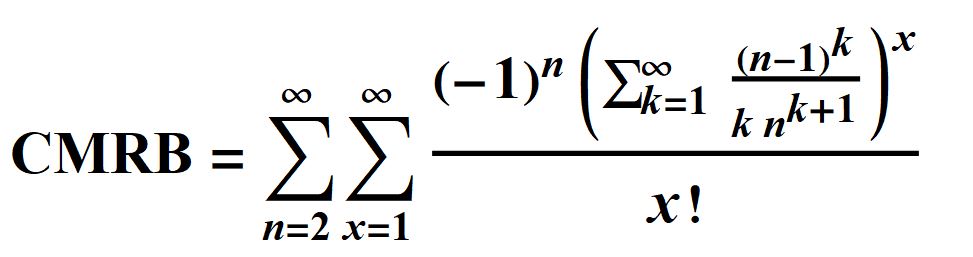
I found the following equation for CMRB (great for integer arithmetic because
(1-1/n)^k=(n-1)^k/n^k. )
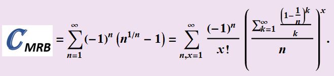
So, using only integers, and sufficiently large ones in place of infinity, we can use
See
In[1]:= Timing[m=NSum[(-1)^n (n^(1/n)-1),{n,1,Infinity},WorkingPrecision->200,Method->"AlternatingSigns"]][[1]]

Out[1]= 0.086374

In[2]:= Timing[m-NSum[(-1)^n/x! (Sum[((-1 + n)^k) /(k n^(1 + k)), {k, 1, Infinity}])^ x, {n, 2, Infinity}, {x, 1,100}, Method -> "AlternatingSigns",  WorkingPrecision -> 200, NSumTerms -> 100]]

Out[2]= {17.8915,-2.2*^-197}
It is very much slower, but it can give a rational approximation (p/q), like in the following.
In[3]:= mt=Sum[(-1)^n/x! (Sum[((-1 + n)^k) /(k n^(1 + k)), {k, 1,500}])^ x, {n, 2,500}, {x, 6}];

In[4]:= N[m-mt]

Out[4]= -0.00602661

In[5]:= Head[mt]

Out[5]= Rational
Compared to the NSum formula for m, we see
In[6]:= Head[m]

Out[6]= Real
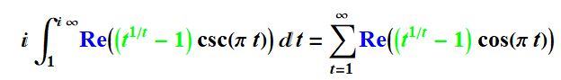
On 9/19/2021
I found the following quality of CMRB.
On 9/5/2021
I added the following MRB constant integral over an unusual range.
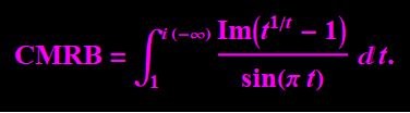
See proof in this link here.
On Pi Day, 2021, 2:40 pm EST,
I added a new MRB constant integral.


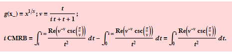
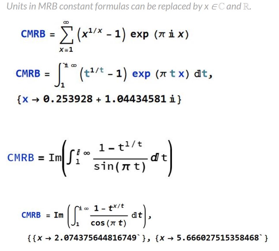
We see many more integrals for CMRB.
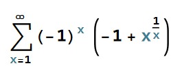
We can expand
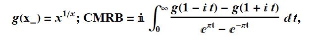 into the following.

xx = 25.65665403510586285599072933607445153794770546058072048626118194\
90097321718621288009944007124739159792146480733342667`100.;


g[x_] = x^(xx/
    x); I NIntegrate[(g[(-t I + 1)] - g[(t I + 1)])/(Exp[Pi t] -
           Exp[-Pi t]), {t, 0, Infinity}, WorkingPrecision -> 100]

 (*
0.18785964246206712024851793405427323005590309490013878617200468408947\
72315646602137032966544331074969.*)
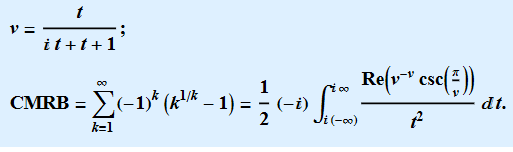
Expanding upon the previously mentioned
we get the following set of formulas that all equal CMRB:
Let
x= 25.656654035105862855990729 ...
along with the following constants (approximate values given)
{u = -3.20528124009334715662802858},
{u = -1.975955817063408761652299},
{u = -1.028853359952178482391753},
{u = 0.0233205964164237996087020},
{u = 1.0288510656792879404912390},
{u = 1.9759300365560440110320579},
{u = 3.3776887945654916860102506},
{u = 4.2186640662797203304551583} or
$
u = \infty .$
then
See
this notebook from the wolfram cloud
and this notebook
for justification.
Also, there is symmetry between the local extrema of the left half of the plane with the right.
2020 and before:
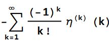
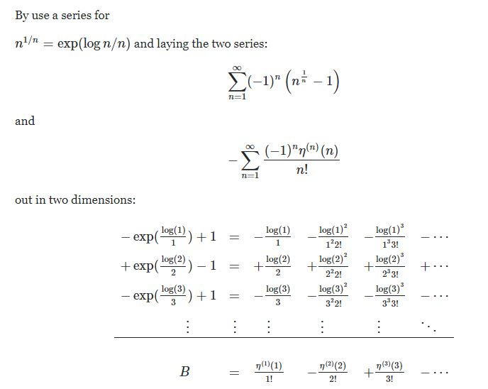
Also, in terms of the Euler-Riemann zeta function,
CMRB =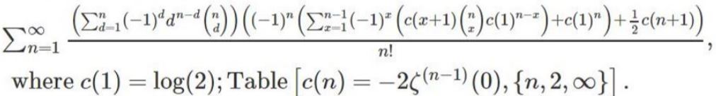
Furthermore, as  ,
,
according to user90369 at Stack Exchange, CMRB can be written as the sum of zeta derivatives similar to the eta derivatives discovered by Crandall.
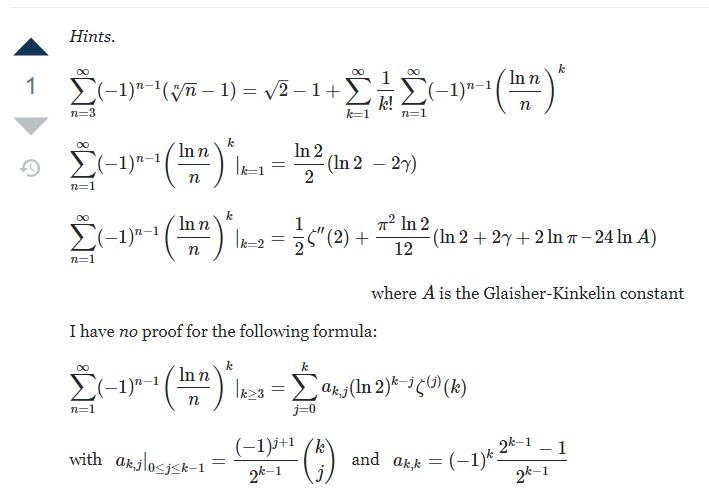 Information about η(j)(k) please see e.g. this link here, formulas (11)+(16)+(19).
In the light of the parts above, where
CMRB
= 
= 
= 
 as well as
 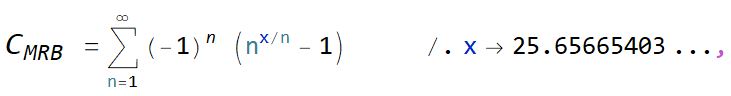 an internet scholar going by the moniker "Dark Malthorp" wrote:
Primary Proof 1
CMRB= , based on
CMRB
is proven below by an internet scholar going by the moniker "Dark Malthorp."
Primary Proof 2
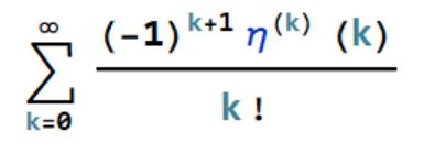
 denoting the kth derivative of the Dirichlet eta function of k and 0 respectively,
was first discovered in 2012 by Richard Crandall of Apple Computer.
denoting the kth derivative of the Dirichlet eta function of k and 0 respectively,
was first discovered in 2012 by Richard Crandall of Apple Computer.
The left half is proven below by Gottfried Helms and it is proven more rigorously considering the conditionally convergent sum,
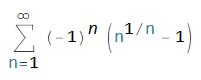
 below that. Then the right half is a Taylor expansion of eta(s) around s = 0.
At
https://math.stackexchange.com/questions/1673886/is-there-a-more-rigorous-way-to-show-these-two-sums-are-exactly-equal,
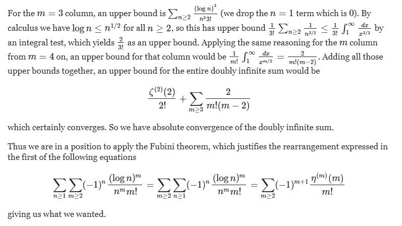
it has been noted that "even though one has cause to be a little bit wary around formal rearrangements of conditionally convergent sums (see the Riemann series theorem), it's not very difficult to validate the formal manipulation of Helms. The idea is to cordon off a big chunk of the infinite double summation (all the terms from the second column on) that we know is absolutely convergent, which we are then free to rearrange with impunity. (Most relevantly for our purposes here, see pages 80-85 of this document, culminating with the Fubini theorem which is essentially the manipulation Helms is using.)"
Primary Proof 3
Here is proof of a faster converging integral for its integrated analog (The MKB constant) by Ariel Gershon.
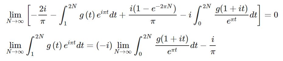
g(x)=x^(1/x), M1=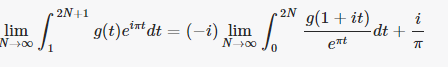
Which is the same as
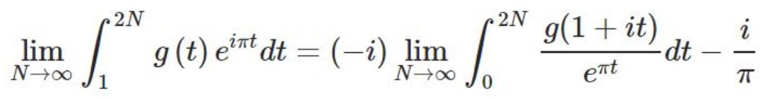 because changing the upper limit to 2N + 1 increases MI by 2i/?.
MKB constant calculations have been moved to their discussion at http://community.wolfram.com/groups/-/m/t/1323951?ppauth=W3TxvEwH .
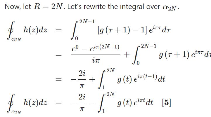
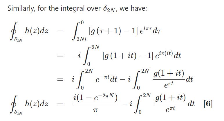
Plugging in equations [5] and [6] into equation [2] gives us:
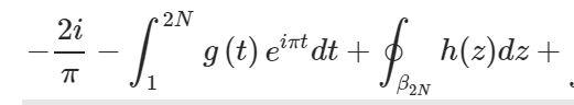
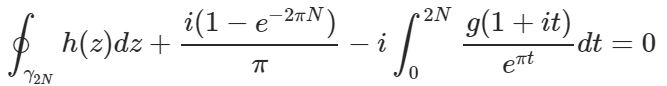
Now take the limit as N-> infinity and apply equations [3] and [4] :
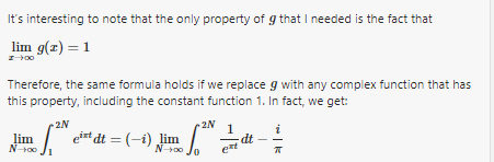
 He went on to note that
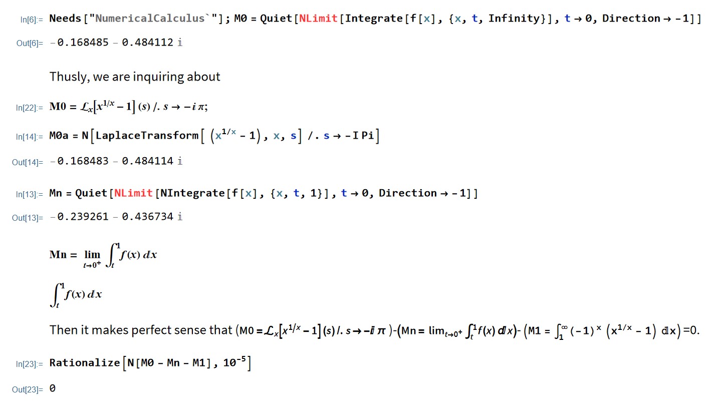
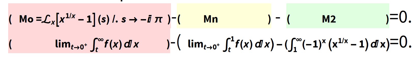
I wondered about the relationship between CMRB and its integrated analog and asked the following.
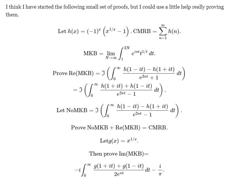 So far I came up with
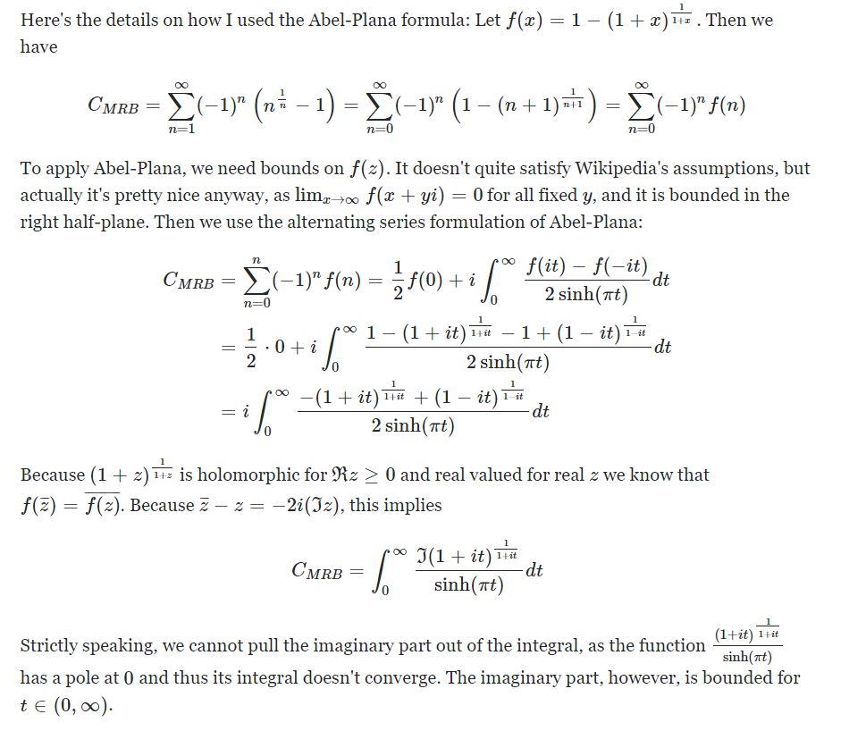
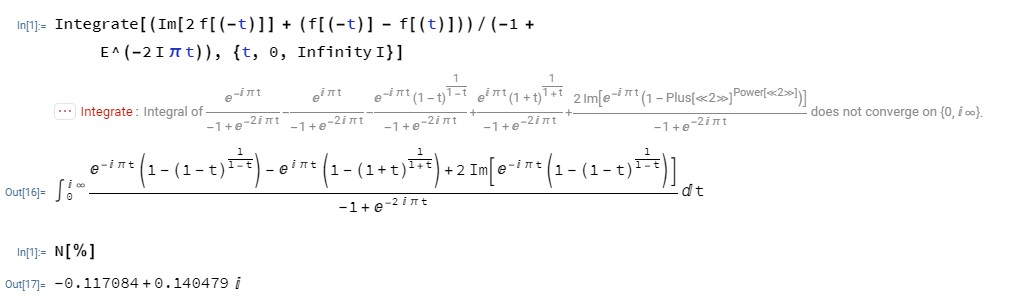
Another relationship between the sum and integral that remains more unproven than I would like is
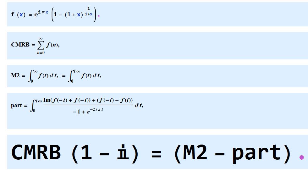
f[x_] = E^(I \[Pi] x) (1 - (1 + x)^(1/(1 + x)));
CMRB = NSum[f[n], {n, 0, Infinity}, WorkingPrecision -> 30,
   Method -> "AlternatingSigns"];
M2 = NIntegrate[f[t], {t, 0, Infinity I}, WorkingPrecision -> 50];
part = NIntegrate[(Im[2 f[(-t)]] + (f[(-t)] - f[(t)]))/(-1 +
      E^(-2 I \[Pi] t)), {t, 0, Infinity I}, WorkingPrecision -> 50];
CMRB (1 - I) - (M2 - part)
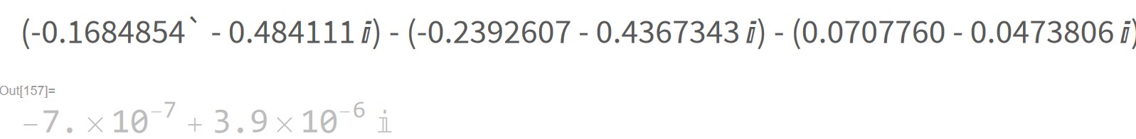
gives
6.10377910^-23 - 6.10377910^-23 I.
Where the integral does not converge, but Mathematica can give it a value:
Update 2015
Here is my mini-cluster of the fastest 3 computers (the MRB constant supercomputer 0) mentioned below:
The one to the left is my custom-built extreme edition 6 core and later with an 8 core 3.4 GHz Xeon processor with 64 GB 1666 MHz RAM..
The one in the center is my fast little 4-core Asus with 2400 MHz RAM.
Then the one on the right is my fastest -- a Digital Storm 6 core overclocked to 4.7 GHz on all cores and with 3000 MHz RAM.

 see notebook
Likewise, Wolfram Alpha here says
It also adds
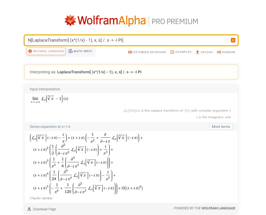
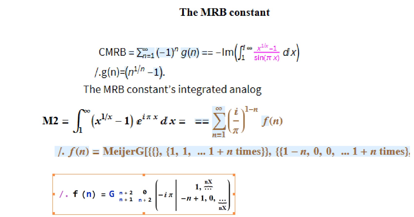
Interestingly,
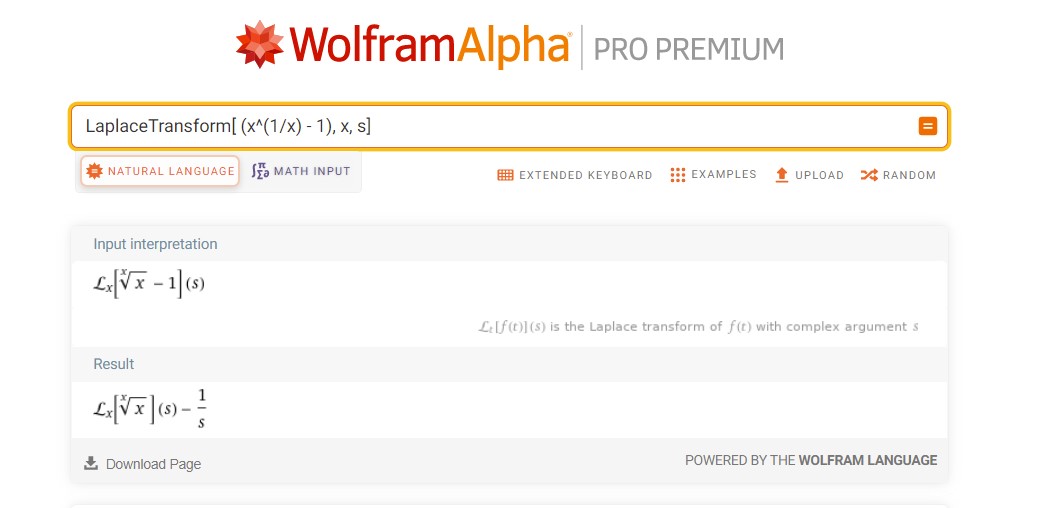
That has the same argument,
 ,
as the MeijerG transformation of CMRB.
,
as the MeijerG transformation of CMRB.
The next reply should say "
§13.
MRB Constant Records,"
If not refresh the page to see them.


