About a year ago, Marco Thiel showed us how to read high resolution weather data from Netatmo. In another wonderful post, aftermath of the solar eclipse, he imported data from his own Netatmo weather station. This fact, along with the possibility of connecting Netatmo to Data Drop, is what convinced me to get my own Netatmo weather station.

In this post I want to share with you some tips to interpret physical quantities using the function SemanticImport. Netatmo is saving the station's data to the Cloud but there is an advanced option to download the station data as a CSV/XLS file:

My indoor station data for September is being attached in this post as cvs file. Once it has been downloaded, save it with the (attached) notebook and follow these simple steps:

SetDirectory[NotebookDirectory[]];

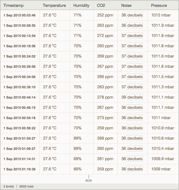
Before using SemanticImport, I usually take a look at the first few rows of the cvs document to see how it is structured:

Grid[Take[Import["Indoor_9-2015.csv"], 5], Frame -> All]

I'm based in Barcelona so the time zone is 2:

$TimeZone = 2

In SemanticImport there is an option called ExcludedLines, I use it to remove the first three rows. Then I use an association to take the columns {"Timestamp", "Temperature", "Humidity", "CO2", "Noise", "Pressure"} and to specify the type of interpreter to be applied at each column. Finally, once the SemanticImport returns a Dataset, I apply the function FromUnixTime to timestamps to convert them into DateObjects:

indoor = SemanticImport["Indoor_9-2015.csv",
   <|"Timestamp" -> Automatic,
    "Temperature" -> 
     Restricted["StructuredQuantity", "DegreesCelsius"], 
    "Humidity" -> Restricted["StructuredQuantity", "Percent"], 
    "CO2" -> Restricted["StructuredQuantity", "PartsPerMillion"], 
    "Noise" -> Restricted["StructuredQuantity", "dB"], 
    "Pressure" -> Restricted["StructuredQuantity", "Millibars"] |>,
   ExcludedLines -> Range[3]][All, {"Timestamp" -> FromUnixTime}]

Having this as structured dataset it makes it easy to compute all sort of things:

indoor[MinMax, "Temperature"]

indoor[DateListPlot, {"Timestamp", "CO2"}]

The symbolic character of the Wolfram Language allows me to add any degree of sophistication. For example here I grouped the measurements by hour:

byHour = GroupBy[indoor, DateValue[#Timestamp, "Hour"] &]

I find this specially convenient if one wants to know what an average day looks like. Here is the ListLinePlot of CO2 concentration in my apartment air:

ListLinePlot[byHour[All, All, "CO2"][All, Mean],
 ColorFunction -> "CMYKColors",
 Filling -> 700,
 AxesLabel -> Automatic,
 Mesh -> All,
 Ticks -> {Range[0, 24, 1], Automatic},
 GridLines -> {Range[0, 24, 1]}]

CO2 concentration rises up over night due to inexistent air exchange, and it goes down in the morning when windows are opened. Around 2pm there is a smaller peak and I suspect that it is caused by the midday rush hour when the noise level rises up:

ListLinePlot[byHour[All, All, "Noise"][All, Mean],
 ColorFunction -> "CMYKColors",
 Filling -> 80,
 AxesLabel -> Automatic,
 Mesh -> All,
 Ticks -> {Range[0, 24, 1], Automatic},
 GridLines -> {Range[0, 24, 1]}]

The driest hour of the day is found at 12pm:

ListLinePlot[byHour[All, All, "Humidity"][All, Mean], 
 ColorFunction -> "RedBlueTones", Filling -> 2000, 
 AxesLabel -> Automatic, Mesh -> All, 
 Ticks -> {Range[0, 24, 1], Automatic}, 
 GridLines -> {Range[0, 24, 1]}]

And the coldest at 9am:

ListLinePlot[byHour[All, All, "Temperature"][All, Mean], 
 ColorFunction -> "TemperatureMap", Filling -> 2000, 
 AxesLabel -> Automatic, Mesh -> All, 
 Ticks -> {Range[0, 24, 1], Automatic}, 
 GridLines -> {Range[0, 24, 1]}]

What surprised me the most was that the pressure measurements clearly showed the existence of a rhythmic semidiurnal pressure variation, a not fully understood phenomenon known as the atmospheric tide.

p = Mean[indoor[All, "Pressure"]];
ListLinePlot[byHour[All, All, "Pressure"][All, Mean[#] - p &],
 ColorFunction -> "Pastel",
 AxesLabel -> Automatic, AxesOrigin -> {0, -.7}, 
 PlotStyle -> AbsoluteThickness[4], Mesh -> All,
 Ticks -> {Range[0, 24, 1], Automatic},
 GridLines -> {Range[0, 24, 1], Range[-.6, .6, .6]}, 
 PlotLegends -> Placed[Style["The atmospheric tide at Barcelona, 24h", "Text"], Top]]

This post has looked at how to import and analyze a dataset, but there are many other things that can be done. For instance, one could upload this data to the Wolfram Data Drop platform, and then analyze the corresponding Databin:

bin = CreateDatabin[<|"Name" -> "September 2015"|>];
(* Notice that the data must be uploaded in smaller chunks to avoid overloading Data Drop's API *)
DatabinUpload[bin, #] & /@Partition[Normal[indoor], 3000, 3000, 1, Nothing]

DateListPlot, Mean, etc., can be directly applied to a Databin:

DateListPlot[Databin["7vjapOnA"]]

Dataset@N@Mean@Databin["7vjapOnA"]

All the best from Barcelona,

Bernat

Attachments: