One thing that I suggest you to take into account is the color profile with which your image is encoded. For the applications in physics it is crucial whether the color intensity values of your image are proportional to the actual light intensities recorded by your photoelectronic device or they are transformed into a "gamma-corrected" and hence non-additive derivatives. With non-additive values any interpolation scheme produces misleading results.

Antonio,

Here is a solution based on the Bresenham's algorithm implemented by halirutan:

bresenham[p0_, p1_] := Module[{dx, dy, sx, sy, err, newp},
  {dx, dy} = Abs[p1 - p0];
  {sx, sy} = Sign[p1 - p0];
  err = dx - dy;
  newp[{x_, y_}] := 
   With[{e2 = 2 err}, {If[e2 > -dy, err -= dy; x + sx, x], 
     If[e2 < dx, err += dx; y + sy, y]}];
  NestWhileList[newp, p0, # =!= p1 &, 1]
];

Since Bresenham's algorithm requires integer pixel positions for both ends of the line we have to snap the line to the pixel grid in the coordinate system used by PixelValue which differs from the standard image coordinate system by 1/2:

\[Alpha] = Pi/4;
radius = 300;

crcl = ComponentMeasurements[RegionBinarize[Dilation[img, 3], {{600, 440}}, 0.5], 
   "Centroid"];
(* centroid in the standard image coordinate system *)
center = 1 /. crcl;
(*integer position of the central pixel in the coordinate system used by PixelValue*)
centralPixelPosition = Round@N[center + 1/2];
(*integer position of the ending pixel in the coordinate system used by PixelValue*)
endingPixelPosition = Round@N[AngleVector[centralPixelPosition, {radius, \[Alpha]}]];
radialPixelPositionsBresenham = bresenham[centralPixelPosition, endingPixelPosition];
radialProfileBresenham = 
  Transpose[{Map[N@EuclideanDistance[centralPixelPosition, #] &, 
     radialPixelPositionsBresenham], PixelValue[img, radialPixelPositionsBresenham]}];

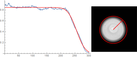
model = a/b Erfc[(-x + \[Mu])/(Sqrt[2] \[Sigma])];
fit = FindFit[radialProfileBresenham, model, {a, b, \[Mu], \[Sigma]}, x];
Row[{Show[ListLinePlot[radialProfileBresenham, ImageSize -> Medium], 
   Plot[model /. fit, {x, 0, radius}, PlotStyle -> Red, PlotRange -> All, 
    Evaluated -> True]], 
  Show[img, Epilog -> {Red, Thickness[.01], 
     Arrow[{centralPixelPosition - 1/2, endingPixelPosition - 1/2}], 
     Circle[centralPixelPosition - 1/2, radius]}, ImageSize -> Small]}]

Also find attached updated version of your Notebook.

Attachments:

Dear Alexey, All solutions are good. If you allow me I would like to add one more requirement. I have tried, but my knowledge is still not enough to solve it in a short time. It would be interesting if it were possible to use the image center (prior calculation of the centroid). Also interesting would finish line profile in a circle of radius r. I have tried adapt a small routine in attachment without success until now. Thank you anyway

Antonio

Attachments:

Hi Antonio,

Here is one approach:

\[Alpha] = Pi/3;
id = ImageDimensions[img];
pr = {0, #} & /@ id;
center = Mean /@ pr;
gr = Graphics[{White, AbsoluteThickness[1], 
    Line[{center, AngleVector[center, {Norm[id], \[Alpha]}]}]}, Background -> Black, 
   PlotRangePadding -> None, ImageSize -> id, PlotRange -> pr, AspectRatio -> Automatic];
mask = Binarize@Rasterize[Style[gr, Antialiasing -> False], "Image"];
radialProfile = 
  PixelValue[img, SortBy[PixelValuePositions[mask, 1], N@EuclideanDistance[center, #] &]];
Row[{ListLinePlot[radialProfile, ImageSize -> Medium], Show[img, gr /. White -> Red]}]

I also attach updated version of your Notebook to this post.

Attachments: