The international year of light has just drawn to an end. From 4-6 February the closing ceremony took place in Merida, Yukatan.

GeoGraphics[GeoMarker[Entity["City", {"Merida", "Yucatan", "Mexico"}]], GeoRange -> Quantity[3000, "Kilometers"], GeoBackground -> "ReliefMap"]

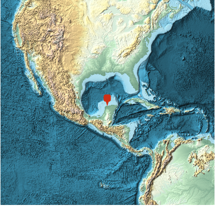
The international Year of Light was a global initiative of the United Nations to celebrate light and light based technologies. Mathematica's built-in Wikipedia data contains detailed information on the Year of Light; here is the first sentence of the article.

TextSentences[WikipediaData["Year of Light"]][[1]]

The International Year of Light and Light-based Technologies, 2015 (IYL 2015) is a United Nations observance that aims to raise awareness of the achievements of light science and its applications, and its importance to humankind.

I am planning to write three posts to show how the Wolfram Language, its wealth of data, and connected devices can be used to keep the year of light alive at your home. In this first part, I will use a spectrometer, connect it to the Wolfram Language, and try to "see the world in a different light". It turns out that the Wolfram Language will be as important as the hardware for this project.

Light is key to life on earth and sight is a key sense; most of the information our brains process comes from our vision. When the first organism developed primitive vision, that was an enormous evolutionary advantage, allowing them to escape preditors and localise prey. Light plays a crucial role in our modern lifes - most likely the information on this very website was delivered to you using optical fibres and light. Light also allows us to study everything from the smallest particles up to the farthest reaches of the universe.

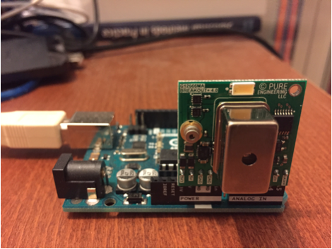
In the 17th century Sir Isaac Newton introduced the word "spectrum" into optics, referring to the range of colours observed whey light passed through a prism. Today spectrometers are used in many scientific labs to study everything from molecules to the light of stars. In this Community several posts have described the construction of spectrometers and raspberry pi spectrometers. For this blog I will use a commercial, small spectrometer, the C12666MA Micro-Spectrometer, that attaches to an Arduino Uno. Hooking it up to the Arduino is trivial as the pins nicely align.

I will first upload the following code to the Arduino:

// This code is a modified from the original sketch from Peter Jansen
// https://github.com/tricorderproject/arducordermini
// This code removes the external ADC and uses the internal ADC instead. 
// also this code just prints the output to csv output to the terminal. 

#define SPEC_GAIN        A0
//#define SPEC_EOS         NA
#define SPEC_ST          A1
#define SPEC_CLK         A2
#define SPEC_VIDEO       A3
#define WHITE_LED        A4
#define LASER_404        A5

#define SPEC_CHANNELS    256
uint16_t data[SPEC_CHANNELS];

void setup() {

  //pinMode(SPEC_EOS, INPUT);
  pinMode(SPEC_GAIN, OUTPUT);
  pinMode(SPEC_ST, OUTPUT);
  pinMode(SPEC_CLK, OUTPUT);

  pinMode(WHITE_LED, OUTPUT);
  pinMode(LASER_404, OUTPUT);
  digitalWrite(WHITE_LED, LOW);
  digitalWrite(LASER_404, LOW);


  //digitalWrite(WHITE_LED, HIGH);
  //digitalWrite(LASER_404, HIGH);

  digitalWrite(SPEC_GAIN, HIGH);
  digitalWrite(SPEC_ST, HIGH);
  digitalWrite(SPEC_CLK, HIGH);
  digitalWrite(SPEC_GAIN, HIGH); //LOW Gain
  //digitalWrite(SPEC_GAIN, LOW); //High Gain

  //Serial.begin(9600);
  Serial.begin(115200);
}

void readSpectrometer()
{
  //int delay_time = 35;     // delay per half clock (in microseconds).  This ultimately conrols the integration time.
  int delay_time = 1;     // delay per half clock (in microseconds).  This ultimately conrols the integration time.
  int idx = 0;
  int read_time = 35;      // Amount of time that the analogRead() procedure takes (in microseconds) (different micros will have different times) 
  int intTime = 5; 
  int accumulateMode = false;
  int i;

  // Step 1: start leading clock pulses
  for (int i = 0; i < SPEC_CHANNELS; i++) {
    digitalWrite(SPEC_CLK, LOW);
    delayMicroseconds(delay_time);
    digitalWrite(SPEC_CLK, HIGH);
    delayMicroseconds(delay_time);
  }

  // Step 2: Send start pulse to signal start of integration/light collection
  digitalWrite(SPEC_CLK, LOW);
  delayMicroseconds(delay_time);
  digitalWrite(SPEC_CLK, HIGH);
  digitalWrite(SPEC_ST, LOW);
  delayMicroseconds(delay_time);
  digitalWrite(SPEC_CLK, LOW);
  delayMicroseconds(delay_time);
  digitalWrite(SPEC_CLK, HIGH);
  digitalWrite(SPEC_ST, HIGH);
  delayMicroseconds(delay_time);

  // Step 3: Integration time -- sample for a period of time determined by the intTime parameter
  int blockTime = delay_time * 8;
  long int numIntegrationBlocks = ((long)intTime * (long)1000) / (long)blockTime;
  for (int i = 0; i < numIntegrationBlocks; i++) {
    // Four clocks per pixel
    // First block of 2 clocks -- measurement
    digitalWrite(SPEC_CLK, LOW);
    delayMicroseconds(delay_time);
    digitalWrite(SPEC_CLK, HIGH);
    delayMicroseconds(delay_time);
    digitalWrite(SPEC_CLK, LOW);
    delayMicroseconds(delay_time);
    digitalWrite(SPEC_CLK, HIGH);
    delayMicroseconds(delay_time);

    digitalWrite(SPEC_CLK, LOW);
    delayMicroseconds(delay_time);
    digitalWrite(SPEC_CLK, HIGH);
    delayMicroseconds(delay_time);
    digitalWrite(SPEC_CLK, LOW);
    delayMicroseconds(delay_time);
    digitalWrite(SPEC_CLK, HIGH);
    delayMicroseconds(delay_time);
  }


  // Step 4: Send start pulse to signal end of integration/light collection
  digitalWrite(SPEC_CLK, LOW);
  delayMicroseconds(delay_time);
  digitalWrite(SPEC_CLK, HIGH);
  digitalWrite(SPEC_ST, LOW);
  delayMicroseconds(delay_time);
  digitalWrite(SPEC_CLK, LOW);
  delayMicroseconds(delay_time);
  digitalWrite(SPEC_CLK, HIGH);
  digitalWrite(SPEC_ST, HIGH);
  delayMicroseconds(delay_time);

  // Step 5: Read Data 2 (this is the actual read, since the spectrometer has now sampled data)
  idx = 0;
  for (int i = 0; i < SPEC_CHANNELS; i++) {
    // Four clocks per pixel
    // First block of 2 clocks -- measurement
    digitalWrite(SPEC_CLK, LOW);
    delayMicroseconds(delay_time);
    digitalWrite(SPEC_CLK, HIGH);
    delayMicroseconds(delay_time);
    digitalWrite(SPEC_CLK, LOW);

    // Analog value is valid on low transition
    if (accumulateMode == false) {
      data[idx] = analogRead(SPEC_VIDEO);
    } else {
      data[idx] += analogRead(SPEC_VIDEO);
    }
    idx += 1;
    if (delay_time > read_time) delayMicroseconds(delay_time - read_time);   // Read takes about 135uSec

    digitalWrite(SPEC_CLK, HIGH);
    delayMicroseconds(delay_time);

    // Second block of 2 clocks -- idle
    digitalWrite(SPEC_CLK, LOW);
    delayMicroseconds(delay_time);
    digitalWrite(SPEC_CLK, HIGH);
    delayMicroseconds(delay_time);
    digitalWrite(SPEC_CLK, LOW);
    delayMicroseconds(delay_time);
    digitalWrite(SPEC_CLK, HIGH);
    delayMicroseconds(delay_time);
  }

  // Step 6: trailing clock pulses
  for (int i = 0; i < SPEC_CHANNELS; i++) {
    digitalWrite(SPEC_CLK, LOW);
    delayMicroseconds(delay_time);
    digitalWrite(SPEC_CLK, HIGH);
    delayMicroseconds(delay_time);
  }
}

void print_data()
{
  for (int i = 0; i < SPEC_CHANNELS; i++) 
  {
    Serial.print(data[i]);
    Serial.print(',');
  }
  Serial.print("\n");
}

void loop() 
{
//  digitalWrite(LASER_404, HIGH);
//  readSpectrometer();
//  digitalWrite(LASER_404, LOW);
//  print_data();
//  delay(10);

//  digitalWrite(WHITE_LED, HIGH);
//  readSpectrometer();
//  digitalWrite(WHITE_LED, LOW);
//  print_data();
//  delay(10);

  readSpectrometer();
  print_data();
  delay(10);   
}

The Arduino code is quite long and I first thought to only attach it to the post, but there is a particular line which is important. In the "void readSpectrometer()" part there is the line

int intTime = 5; 

which allows you to set the integration time, i.e. the exposure time. That is a very important parameter to get optimal results. With the new features of the Wolfram Language and in particular with the Arduino Device Connection it is possible to adjust the exposure from within the Wolfram Language code. For this post this is not really necessary, so I will save that for another day.

Connecting the Arduino-Spectrometer duo to Mathematica is trivial. Here I connect it to an OSX system.

mySpectrometer = DeviceOpen["Serial", {Quiet[FileNames["tty.usb*", {"/dev"}, Infinity]][[1]], "BaudRate" -> 115200}]

This piece of code

Quiet[FileNames["tty.usb*", {"/dev"}, Infinity]][[1]]

facilitates the connection as it detects the correct device automatically. We can now start collecting data like so:

data = Table[Pause[2]; ToExpression /@ StringSplit[FromCharacterCode[SplitBy[DeviceReadBuffer[mySpectrometer], # == 10 &][[-2]]], ","], {i, 6}];

This data aquisition code actually measures 6 spectra and pauses for 2 seconds between individual measurements. These repeated measurements decrease the noise of the measurements. The measurement procedure is very straight foward. You point the spectrometer at an object and execute the data aquisition. Let's fist look at the spectrum of a fluorescent light bulb.

ListLinePlot[N@Mean[Select[data, Length[#] == 256 &]], PlotRange -> All]

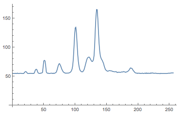
There are several peaks that we will try to understand a little bit later. The x-axis shows 256 bins which represent the different colours, i.e. frequencies. The y-axis shows the count, i.e. the intensity of that frequency band. In oder to be able to interpret the results we first need to calibrate the spectrometer. Here is a link to a table which contains calibration information for various versions of the spectrometer. It turns out that the calibration is performed using a 5th order polynomial; the repective coefficients are given in the calibration table. For my particular spectrometer I obtain:

a0 = 3.170083173*10^2;
b1 = 2.39519817;
b2 = -8.618615345*10^(-4);
b3 = -5.978279712*10^(-6);
b4 = 8.585352787*10^(-9);
b5 = -2.048534811*10^(-12);
wavelength[x_] := a0 + b1  x + b2  x^2 + b3  x^3 + b4*x^4 + b5  x^5

Here is a plot of the calibration curve:

Plot[{wavelength[x]}, {x, 0, 256}]

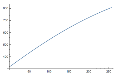
It transforms the number of the bin to the corresponding wavelength. We can not plot the spectrum with the correct x-axis.

datacalibrated = Transpose@{wavelength /@ Range[256], N@Mean[Select[data, Length[#] == 256 &]]};
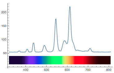
ListLinePlot[datacalibrated, PlotRange -> All]

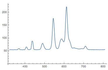
This is much better. This is how a professional spectrum of a fluorescent light bulb looks like:

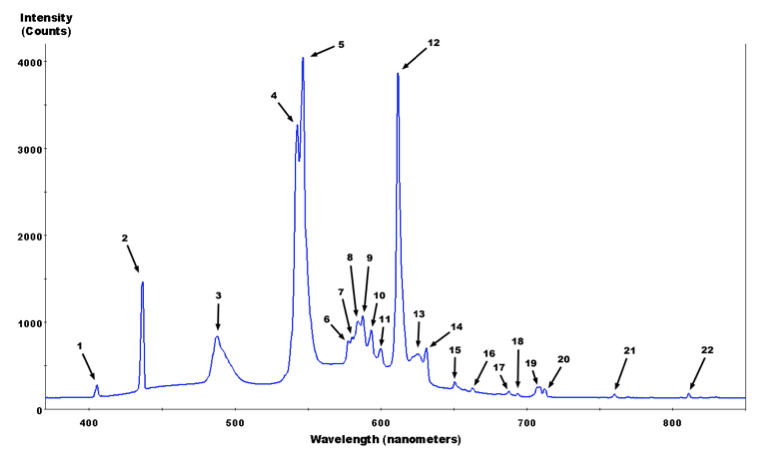
which is taken from the Wikipedia commons. Here is a list of the peaks and what element they correspond to:

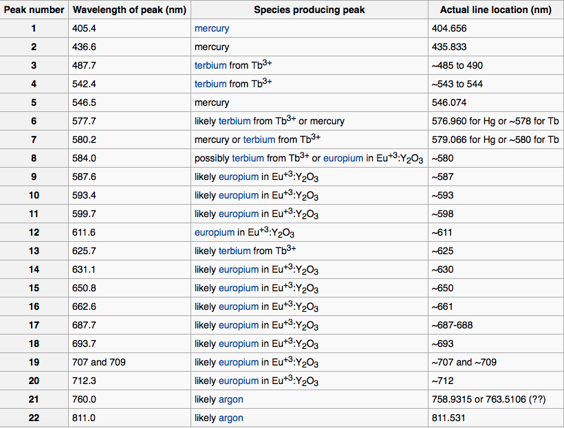
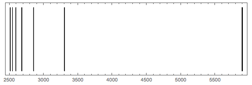
We clearly see the peaks for Mercury, Terbium and Europium. Wolfram|Alpha has a wealth of information about spectral lines and we can use the following line to get it.

WolframAlpha["spectral lines mercury"]

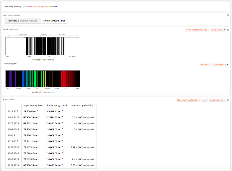
The two dominant lines here are the one at 4046.565 Angstrom and at 4358.335 Angstrom. They correspond to our lines at about 405 nm and 436 nm. Unfortunately, I have failed to extract a list of all relevant spectral lines from Wolfram|Alpha.

Let's try to spice our representation of the spectrum up a bit. It would be nice to have a visual cue as to the colour the different wavelengths correspond to. Mathematica and the Wolfram Language have everything built in to make this task really easy:

ColorData["VisibleSpectrum"][#] & /@ datacalibrated[[All, 1]]

We can now merge this into a band of colours that we can plot with the spectrum.

Graphics[Table[{ColorData["VisibleSpectrum"][datacalibrated[[i, 1]]], Rectangle[{datacalibrated[[i, 1]], 0}, {datacalibrated[[i + 1, 1]],40}]}, {i, 1, Length[datacalibrated] - 1}]]

If we plot this together things start being easier to interpret.

Show[ListLinePlot[datacalibrated, PlotRange -> All], Graphics[Table[{ColorData["VisibleSpectrum"][datacalibrated[[i, 1]]],
     Rectangle[{datacalibrated[[i, 1]], 10}, {datacalibrated[[i + 1, 1]], 40}]}, {i, 1, Length[datacalibrated] - 1}]]]

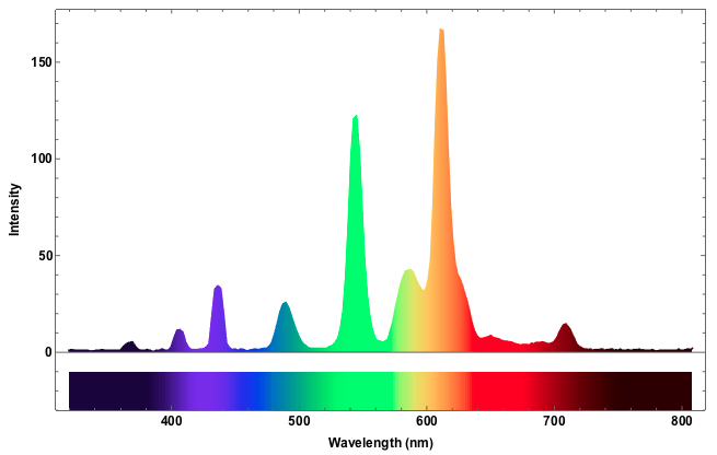
Now there are two more things I want to tweak. First of all there is this off-set of 54; that is a "zero count", i.e. I obtain at least 54 even if there is no signal so I need to subtract that. This number depends on the spectrometer that you have. On a second one I have got that value is different. Also, I would like the lightcurve itself to reflect the colour. The following code achieves that:

Show[ListLinePlot[Evaluate@(Plus[{0., -54.}, #] & /@ datacalibrated), 
  PlotRange -> {All, {-30, All}}, Joined -> True, Frame -> True, 
  ColorFunction -> (Blend["VisibleSpectrum", #1* Differences[datacalibrated[[All, 1]][[{1, -1}]]][[1]] + 
  datacalibrated[[1, 1]]] &), Filling -> Axis, LabelStyle -> Directive[Black, Bold, Medium], 
  FrameLabel -> {"Wavelength (nm)", "Intensity"}], Graphics[Table[{ColorData["VisibleSpectrum"][datacalibrated[[i, 1]]],
     Rectangle[{datacalibrated[[i, 1]], -30}, {datacalibrated[[i + 1, 1]], -10}]}, {i, 1, Length[datacalibrated] - 1}]]]

To identify the spectral lines it is useful to identify maxima of the curve. The following function helps to achieve that:

localMaxPositions = 
  Compile[{{pts, _Real, 1}}, 
   Module[{result = Table[0, {Length[pts]}], i = 1, ctr = 0}, For[i = 2, i < Length[pts], i++, 
     If[pts[[i - 1]] < pts[[i]] && pts[[i + 1]] < pts[[i]],result[[++ctr]] = i]];Take[result, ctr]]];

We can now locate the maxima and plot that on the curve:

dplot = ListLinePlot[datacalibrated, PlotRange -> All];
maxs = ListPlot[Select[Nest[#[[localMaxPositions[#[[All, 2]]]]] &, datacalibrated, 1], #[[2]] > 58.33 &], PlotStyle -> Directive[PointSize[0.015], Green]];
Show[{dplot, maxs}]

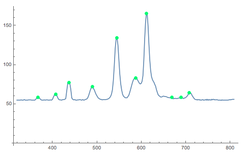
The following function produces a list of the positons of the maxima:

Select[Nest[#[[localMaxPositions[#[[All, 2]]]]] &, datacalibrated, 1], #[[2]] > 58.33 &][[All, 1]]
(*{366.873694406445`,406.4710188519941`,436.1860721777116`,489.\
5449068238321`,544.8439203380104`,587.3854766583466`,610.\
7844904587837`,668.0095922519685`,688.8768717778272`,707.\
3639428495288`}*)

It turns out that there is a packages which contains information about spectral lines, but the elements that we are interested in (Hg, Te, Eu) are not in the database. For elements that are in the database we can compare the measured lines to the ones in the database:

<< ResonanceAbsorptionLines`
ElementAbsorptionMap[Na]

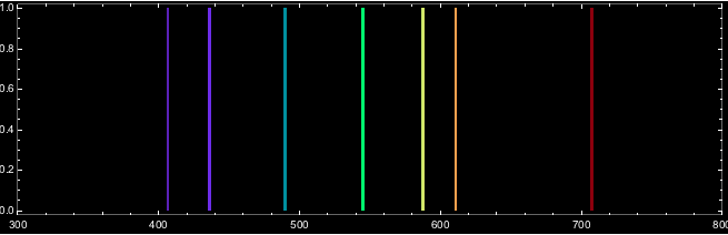
What we can do, however, is to generate - or simulate- an approximatio of the spectral lines we measure. There is a discussion on Stackexchange that shows how to plot an emission spectrum. The following lines are taken from that discussion.

spec[wavelength_, width_] := Flatten[Table[{{x, 0, x}, {x, 1, x}}, {x, wavelength - width, wavelength + width, 0.1}], 1];
ListDensityPlot[
 spec[#, 1] & /@ 
  Select[Nest[#[[localMaxPositions[#[[All, 2]]]]] &, datacalibrated, 
     1], #[[2]] > 59.33 &][[All, 1]], 
 ColorFunction -> ColorData["VisibleSpectrum"], 
 ColorFunctionScaling -> False, AspectRatio -> .3, 
 PlotRange -> {{300, 800}}, 
 FrameTicks -> {Automatic, None, None, None}, 
 FrameTicksStyle -> White, Frame -> True, Background -> Black]

Case Studies

Blue sky

I now measure the spectrum of the blue sky. The measurement was taken late in the year and the sky wasn't the "bluest of blues", but we can still make out some interesting features.

mySpectrometer = 
  DeviceOpen[
   "Serial", {Quiet[FileNames["tty.usb*", {"/dev"}, Infinity]][[1]], 
    "BaudRate" -> 115200}];
datasky = 
  Table[Pause[2]; 
   ToExpression /@ 
    StringSplit[
     FromCharacterCode[
      SplitBy[DeviceReadBuffer[mySpectrometer], # == 10 &][[-2]]], 
     ","], {i, 6}];
a0 = 3.170083173*10^2;
b1 = 2.39519817;
b2 = -8.618615345*10^(-4);
b3 = -5.978279712*10^(-6);
b4 = 8.585352787*10^(-9);
b5 = -2.048534811*10^(-12);
wavelength[x_] := a0 + b1  x + b2  x^2 + b3  x^3 + b4*x^4 + b5  x^5;
datacalibratedsky = 
  Transpose@{wavelength /@ Range[256], N@Mean[Select[datasky, Length[#] == 256 &]]};
Show[ListLinePlot[Evaluate@(Plus[{0., -54.}, #] & /@ datacalibratedsky), 
  PlotRange -> {All, {-30, All}}, Joined -> True, Frame -> True, ColorFunction -> (Blend["VisibleSpectrum", #1*Differences[datacalibratedsky[[All, 1]][[{1, -1}]]][[1]] + datacalibratedsky[[1, 1]]] &), Filling -> Axis, LabelStyle -> Directive[Black, Bold, Medium], FrameLabel -> {"Wavelength (nm)", "Intensity"}], 
 Graphics[Table[{ColorData["VisibleSpectrum"][datacalibratedsky[[i, 1]]], Rectangle[{datacalibratedsky[[i, 1]], -30}, {datacalibratedsky[[i + 1, 1]], -10}]}, {i, 1, Length[datacalibratedsky] - 1}]]]

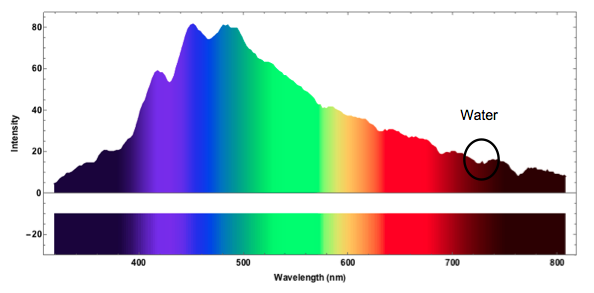
The spectrum clearly shows the "blue" in the sky. It turns out that the marked double dip corresponds to absorption by water.

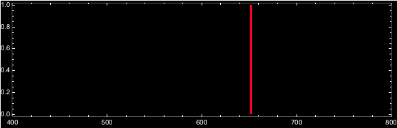
Lasers

Using exactly the same code we can now analyse the spectrum of different lasers - red, green and blue. We can clearly see that the red and green lasers have a very narrow peak within the red and green spectral bands, whereas the blue laser has a much broader peak. This is probably related to how blue laser light is generateed in cheap laser pointers.

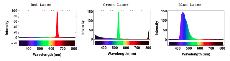
Here is how the spectrum of a red laser would look like:

ListDensityPlot[
 spec[#, 1] & /@ 
  Select[Nest[#[[localMaxPositions[#[[All, 2]]]]] &, datacalibratedlaserr, 1], #[[2]] > 59.33 &][[All, 1]], 
 ColorFunction -> ColorData["VisibleSpectrum"], ColorFunctionScaling -> False, AspectRatio -> .3, 
 PlotRange -> {{400, 800}}, FrameTicks -> {Automatic, None, None, None}, 
 FrameTicksStyle -> White, Frame -> True, Background -> Black] 

Absorption spectrum - green leaf

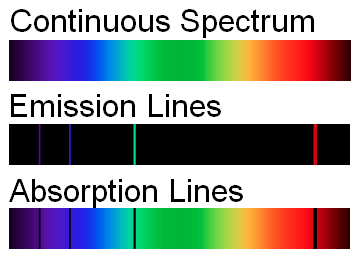
Up to now we have maily discussed emission spectra - apart from some features of the blue sky example. Let's now generate an absorption spectrum. In an emission spectrum a material actively emits radiation/light. In an absoprtion spectrum light that passes through the material.

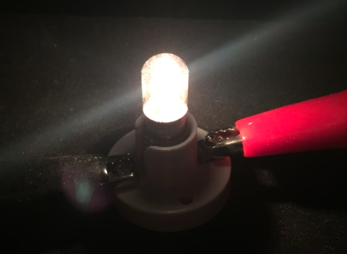
In order to produce a good absorption spectrum we would ideally use a light source that produces a strong continuous spectrum. When I conducted the leaf experiment I only had a very cheap lamp which is usually used by doctors for initial examinations:

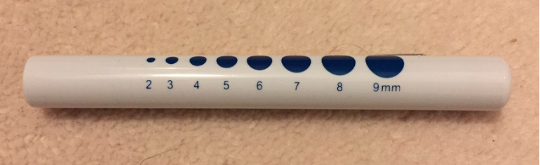
I pointed the lamp at a green leaf and measured the light that shone through. The problem was that the lamp did produce a very poor spectrum heavily biased towards the red frequency range. So in this case study I will first measure the emission spectrum of the lamp and then normalise the absorption spectrum of the leaf. Let's start with the lamp.

mySpectrometer = 
  DeviceOpen[
   "Serial", {Quiet[FileNames["tty.usb*", {"/dev"}, Infinity]][[1]], 
    "BaudRate" -> 115200}];
datalamp = 
  Table[Pause[2]; 
   ToExpression /@ 
    StringSplit[
     FromCharacterCode[
      SplitBy[DeviceReadBuffer[mySpectrometer], # == 10 &][[-2]]], 
     ","], {i, 6}];
a0 = 3.170083173*10^2;
b1 = 2.39519817;
b2 = -8.618615345*10^(-4);
b3 = -5.978279712*10^(-6);
b4 = 8.585352787*10^(-9);
b5 = -2.048534811*10^(-12);
wavelength[x_] := a0 + b1  x + b2  x^2 + b3  x^3 + b4*x^4 + b5  x^5;
datacalibratedlamp = 
  Transpose@{wavelength /@ Range[256], N@Mean[Select[datalamp, Length[#] == 256 &]]};
Show[ListLinePlot[Evaluate@(Plus[{0., -54.}, #] & /@ datacalibratedlamp), 
  PlotRange -> {All, {-30, All}}, Joined -> True, Frame -> True, ColorFunction -> (Blend["VisibleSpectrum", #1*Differences[datacalibratedlamp[[All, 1]][[{1, -1}]]][[1]] + datacalibratedlamp[[1, 1]]] &), Filling -> Axis, 
  LabelStyle -> Directive[Black, Bold, Medium], 
  FrameLabel -> {"Wavelength (nm)", "Intensity"}], 
 Graphics[Table[{ColorData["VisibleSpectrum"][datacalibratedlamp[[i, 1]]], 
 Rectangle[{datacalibratedlamp[[i,1]], -30}, {datacalibratedlamp[[i + 1, 1]], -10}]}, {i, 1,Length[datacalibratedlamp] - 1}]]]

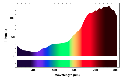
The spectrum is clearly biased to the red freqencies. In the blue/ultraviolet range the light source produces to little output that it will be impossible to determine a reasonable absorption spectrum there. Let's go on to measure the absorption of the leaf.

absorptionleaf = 
  Transpose[{datacalibratedleaf[[All, 1]], (datacalibratedleaf[[All, 2]]/datacalibratedlamp[[All, 2]])}];
Show[ListLinePlot[Evaluate@(Plus[{0., 0.}, #] & /@ absorptionleaf), PlotRange -> {All, {-0.3, 1}}, Joined -> True, Frame -> True, 
  ColorFunction -> (Blend["VisibleSpectrum", #1*Differences[absorptionleaf[[All, 1]][[{1, -1}]]][[1]] + absorptionleaf[[1, 1]]] &), Filling -> Axis, 
  LabelStyle -> Directive[Black, Bold, Medium], FrameLabel -> {"Wavelength (nm)", "Intensity"}], Graphics[Table[{ColorData["VisibleSpectrum"][absorptionleaf[[i, 1]]],Rectangle[{absorptionleaf[[i, 1]], -0.3}, {absorptionleaf[[i + 1,1]], -.1}]}, {i, 1, Length[absorptionleaf] - 1}]]]

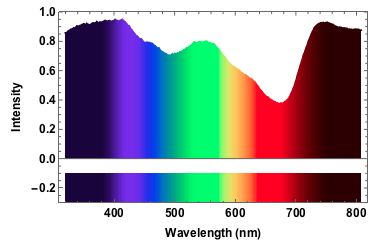
The absorption in the red frequency range stems from chlorophyll; chlorophyll also absorbs in the 400-450nm range which is hard to se here, because of our poor light source. The dip at around 500nm is carotenoids. You can compare that to the spectrum of leaves on this website.

"Black body radiation" - an old fashioned light bulb

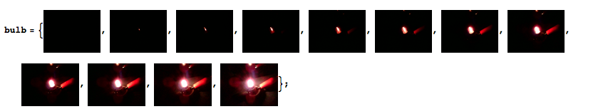
The final example will be of an old fashioned, small light bulb.

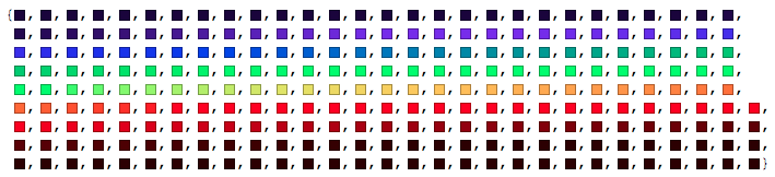
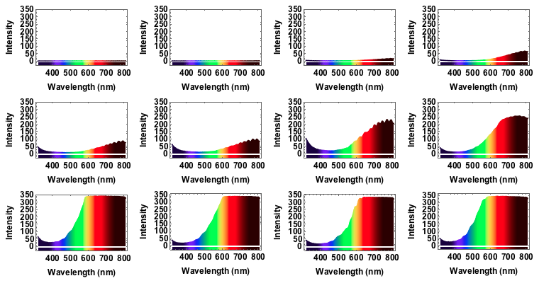
I will use a bench supply to slowly increase the voltage and the current. The filament will go from a red glowing colour to brighter "whiter" colour, but we will see that even for the highest voltage of 12V the spectrum will still be quite different from "white", i.e. uniform. The code is just the same as above. I save all plots for voltages 1V to 12V with increments of 1V in one variable:

specall = {spec1V, spec2V, spec3V, spec4V, spec5V, spec6V, spec7V, spec8V, spec9V, spec10V, spec11V, spec12V}

This can be easily plotted like so:

Grid[Partition[specall, 4]]

We can also animate this:

ListAnimate[specall, AnimationRunTime -> 10]

Note that from 9V onwards the spectrum has max-ed out. When I measured the spectra I took note of the voltage and the corresponding current:

voltageamp = {{1, 0.04}, {2, 0.06}, {3, 0.07}, {4, 0.08}, {5, 0.1}, {6, 0.11}, {7, 0.12}, {8, 0.13}, {9, 0.14}, {10, 0.14}, {11, 0.15}, {12, 0.16}}

I can now represent that with the regression line.

Show[ListPlot[voltageamp, AxesLabel -> {"Volts", "Amps"}, LabelStyle -> Directive[Bold, Medium]], 
 Plot[Evaluate@Fit[voltageamp, {1, x}, x], {x, 0, 12}, PlotStyle -> Red]]

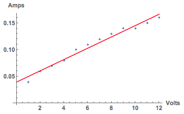
Note the nearly linear increase in current as the voltage increases. Finally, I took photos as the voltage increased.

We now add a little bit of motion to the voltage amp graph:

figvoltsamp = 
  Evaluate@Table[Show[ListPlot[voltageamp, AxesLabel -> {"Volts", "Amps"}, LabelStyle -> Directive[Bold, Medium], 
      Epilog -> {PointSize[Large], Green, Point[voltageamp[[i]]]}], Plot[Evaluate@Fit[voltageamp, {1, x}, x], {x, 0, 12}, PlotStyle -> Red]], {i, 1, 12}];

To finish everything off, we can now animate this:

ListAnimate[GraphicsRow[#, ImageSize -> Full] & /@ Transpose[{specall, bulb, figvoltsamp}]]

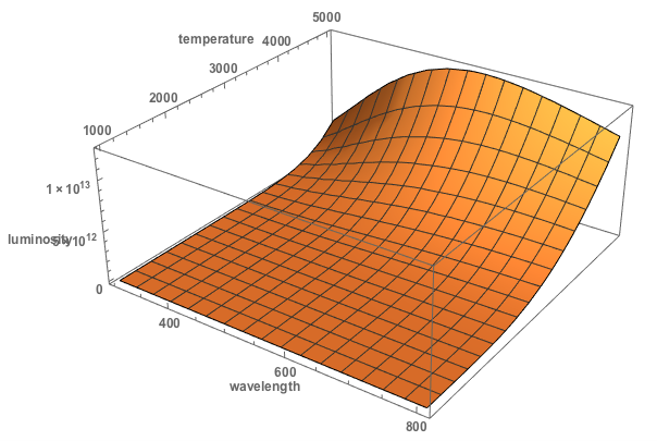
If we were to assume that this is the radiation of a black body, we could use Planck's law:

FormulaData[{"PlanckRadiationLaw", "Wavelength"}]

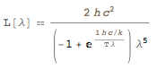
We could plot this as a function of temperature and wavelength

equation = 
  FormulaData[{"PlanckRadiationLaw", "Wavelength"}, {"T" -> Quantity[t, "Kelvins"], 
    "\[Lambda]" -> Quantity[l, "Nanometers"]}];
Plot3D[Quantity[1.191042*^29, ("Pascals")/("Seconds")]/(-1.`16.255 l^5 + 2.71828^(1.438*^7/(l t)) l^5), {l, 300, 808}, {t, 1000, 5000}, PlotRange -> All, 
 AxesLabel -> {"wavelength", "temperature", "luminosity"}, LabelStyle -> Directive[Bold, Medium], ImageSize -> Large]

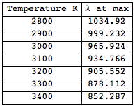
We can also write a little loop to calculate for which wavelength the maximum for different temperatures is reached.

results = {}; Monitor[
 Table[equation2 = FormulaData[{"PlanckRadiationLaw", 
 "Wavelength"}, {"T" -> Quantity[t, "Kelvins"], "\[Lambda]" -> Quantity[l, "Nanometers"]}]; 
  root = FindRoot[D[equation2[[2, 2]], l] == 0, {l, 700}, MaxIterations -> Infinity]; 
  AppendTo[results, {t, root}], {t, 2800, 3400, 100}], t]

This gives the following table:

Grid[Join[{{"Temperature K", "\[Lambda] at max"}}, Transpose[{results[[All, 1]], results[[All, 2, -1, 2]]}]], Frame -> All]

We can plot the relationship between maxium and temperature.

ListLinePlot[Transpose[{results[[All, 1]], results[[All, 2, -1, 2]]}],Mesh -> Full, MeshStyle -> Red, 
 AxesLabel -> {"Temperature", "wavelength at max"}, LabelStyle -> Directive[Bold, Medium], ImageSize -> Large]

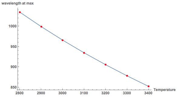
This allows us in principle to estimate the temperature of the filament. Note, that for 8V the maximum is at about 750nm. The graph shows that this corresponds to a temperature higher than 3400K, which is too high for such a small light bulb. So there is still quite some room for improvement... The principle of temperature measurement, by the colour of the sample is realistic.

There are many further projects one could think of. I suppose that with a decent telescope it should be possible to analyse the light of stars for example. Also, the spectrometer works nicely on a Raspberry Pi. It should be quite straight forward to take measurements of say the sky over the day and see how the dominant colours change.

Cheers,

Marco