Message Boards Message Boards

0
|
7713 Views
|
5 Replies
|
2 Total Likes
View groups...
Share
Share this post:

Fitting (x,y) data to model, with more weight at higher y values

Posted 8 years ago

I have some data of capacitance vs frequency for a capacitor. It was measured from 50 MHz to 20 GHz. The capacitance is not fixed with frequency, and I want to fit a 3rd order polynomial to this data. The problem is, its more important that the data is right at high frequencies, and less important at low frequencies. In fact, as a first order approximation, the goodness of fit should be directly proportional to frequency, although I would not say that's optimal, but certainly it needs to fit better at high frequencies, and I can tollerate more errors at low frequencies.

See the attached measurements, which shows frequency (in Hz) on the x-axis and capacitance in Farads on the y-axis.I've attached the raw-data as a text file.

Not only is it more important for the fit to be good at high frequencies, but the measurement errors are almost certainly higher at low frequencies.

enter image description here

Attachments:
POSTED BY: David Kirkby
5 Replies
Posted 8 years ago

I'm deleting what I wrote before in this post, as I realized there's a serious flaw in my argument about the importance of errors being directly proportional to frequency. I will re-write it later.

I like the Manipulate idea. I will look at that.

Dave

POSTED BY: David Kirkby
Posted 8 years ago

Despite my admonishment about "knowing it when you see it", maybe this is a case where one needs to do that (given that your device can handle polynomials and then only up to a 3rd order polynomial - and I assume the device can't take logs or exponentiate the dependent or independent variable?) Using Manipulate might be a good way to see what's possible. If just using data greater than some threshold to estimate the model coefficients, the following might help:

Manipulate[

 (* Get subset of data that is greater than the threshold *)
 cap = Select[capacitance, #[[1]] > threshold &];

 (* Fit the model with the subset of data *)
 lm = LinearModelFit[cap, {x, x^2, x^3}, {x}];

 (* Plot results *)
 Show[
  ListPlot[capacitance, 
   PlotRange -> {Automatic, {8 10^(-14), 1.3 10^(-13)}}],
  ListPlot[cap, PlotStyle -> Red],
  Plot[lm[x], {x, xmin, xmax}, PlotStyle -> Green], ImageSize -> Large
  ],

 {{threshold, 6 10^9, "Threshold"}, xmin, xmax, Appearance -> "Labeled"},
 TrackedSymbols :> {threshold},
 Initialization :> (
   capacitance = 
    Import["derrived-capacitance-data-in-Hz-and-Farads.txt", "CSV"];
   xmin = Min[capacitance[[All, 1]]];
   xmax = Max[capacitance[[All, 1]]])]

Data and fit

POSTED BY: Jim Baldwin
Posted 8 years ago

Hi, I made a mess-up there. The data file I posted was not the raw data, but had been smoothed already. I attach the correct file, which I call "derrived-capacitance-data-in-Hz-and-Farads.txt"

I can be more specific about what I want to do, but it might make it more tricky to understand. I was a bit reluctant to describe it in too much detail, as I thought I'd just make the issue more confusing. But since Jim asked, this describes what I really want to do.

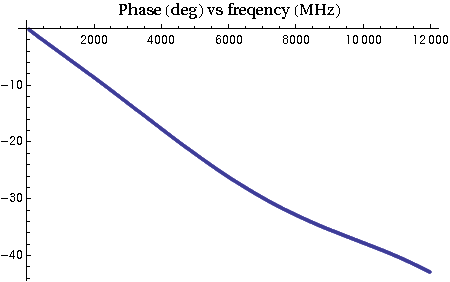
1) Measure a set of phase values, phi up to 12 GHz. These are shown in the file original-phase-data-in-MHz-and-degrees.txt. The first column is frequency in MHz, and the second is the phase in degrees.

This experimentally measured phase values look fairly smooth. Note the phase is almost linear with frequency. Higher frequencies result in larger phase shifts.

2) Compute the capacitance C from that phase data, using the formula. C=-Tan[phase/2]/(100 Pi f) - where phase is in radians and f is in Hz.

That looks rather noisy, and is shown in the file derrived-capacitance-data-in-Hz-and-Farads.txt

It is somewhat puzzling that a fairly clean looking set of phase data results in a rather noisy set of capacitance data.

3) Model the capacitor as a third order polynomial.

4) Varying the frequency from DC to 12 GHz, I want to compute a second set of phase values based on the model of the capacitor. That will be by just re-arranging the above equation. This set of phase data should be quite smooth, as it will be based on a smooth curve for the capacitor.

5) Reduce the RMS error between the original measured phases and the new set based on a third order fit of capacitance.

Fitting over two ranges may be an option, but I'd really like to get one set of data that does a reasonable job over the whole range. Having improved, but separate sets of coefficients for a more restricted frequency range is certainly something I will consider. But the coefficients for the fit must be entered into an instrument which only accepts a 3rd order polynomial fit.

enter image description here

Attachments:
POSTED BY: David Kirkby
Posted 8 years ago

Just to note that one needs to be more specific than just having more weight with the higher frequencies. Otherwise, the goodness-of-fit criterion just becomes "I'll know it when I see it." The weighting function needs to reflect the consequences of the quality of the predictions at the desired locations. That's a choice you need to control rather than some arbitrary algorithm.

One possibility is to toss out all lower frequencies at whatever threshold you declare. Alternatively, one could just give low (but non-zero) weights to points with low frequencies or write a specific weighting function. Below is some code to weight all low frequencies identically with a low weight:

weights = Table[1, {i, Length[xy[[All, 1]]]}];
weights[[Table[i, {i, 300}]]] = 0.01;
nlm = LinearModelFit[xy, {x, x^2, x^3, x^4}, x, Weights -> weights];
Show[Plot[nlm[x], {x, Min[xy[[All, 1]]], Max[xy[[All, 1]]]}, PlotStyle -> {LightGray, Thickness[0.02]}], 
 ListPlot[xy, PlotStyle -> Red]]

Cubic fit

The data you provided is pretty smooth (much smoother than your example above) and it would seem like you could get a pretty good fit for the whole range of frequencies by performing piecewise regression where you have a cubic for the higher frequencies and a separate function (maybe a cubic, too) for the lower frequencies.

POSTED BY: Jim Baldwin
Posted 8 years ago

.

poly1 = Fit[data, {1, x, x^2, x^3}, x]
Show[ListPlot[data, PlotStyle->Red], Plot[poly1, {x, 5.746875*^7, 1.2*^10}]]

g1

chopdata = Select[data, #[[1]] > 4*^9 &];
poly2 = Fit[chopdata, {1, x, x^2, x^3}, x]
Show[ListPlot[data, PlotStyle->Red], Plot[poly2, {x, 5.746875*^7, 1.2*^10}]]

g2

As you lower the chop threshold the quality of the fit above 5 ghz degrades. Choosing some threshold seems necessary.

Another method you might also apply would be to multiply your y values by some "nice" strictly increasing function of frequency, do the fit and then divide the resulting polynomial by that same function. That will increase the weight of the errors in your measurements at higher frequencies. To play strictly by the rules of statistics this is used to make data homoschedastic, but if you are just trying to force a fit in your area of interest you could try this.

POSTED BY: Bill Simpson
Reply to this discussion
Community posts can be styled and formatted using the Markdown syntax.
Reply Preview
Attachments
Remove
or Discard

Group Abstract Group Abstract