This is a brief project which has been spun off from a much larger project on traffic modelling where seeking/steering behaviours and acceleration strategies are modelled to simulate believable agents in transport environments.
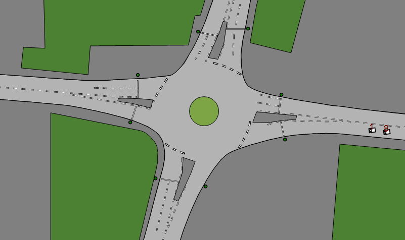
This is a preview of EDI (Extensible Environment Driver Interaction Integrated) simulating traffic flow in a roundabout modelled after St. Machar Drive, Aberdeen, Scotland. It still needs some adjustments though.
A planned feature is to incorporate detection and resolution of collisions between vehicles and so the following began as a experiment. Ultimately, a 1D harmonic oscillator modelled after rigid body collisions was created and demonstrates characteristics found in a similar system but modelled after a different approach using the Intelligent Driver Model.
Collision Detection - Axis Aligned Bounding Boxes (AABB)
Video Game Physics Tutorial - Part II: Collision Detection for Solid Objects
We need a quick way of determining instances and identities of overlapping objects. Here's the basic principal:
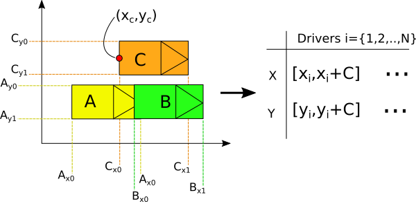
The projection of each object onto its respective axes form intervals. The intersection of any two dissimilar intervals for both axes denotes a collision. As were only dealing with copies of the same object, the length of every interval is constant thus is parameterised by the cars end-point and so makes for a simple function which generates an array of intervals based on the current position of all cars at a time T (in this case, held in testPositions). $\Sigma$ and $\sigma$ are variables set by the user, 15 is the length of each car. Added up, they form the constant interval length.
    boundsMatrix = {
        Interval[{# - \[CapitalSigma], # + 15 + \[Sigma]}] & /@ #[[All,
          1]],
        Interval[{# - 7, # + 7}] & /@ #[[All, 2]]
        } &(* [testPositions] *);
In the diagram, A and B have collided since the intersection of intervals formed on the X and Y axes respectively are non-empty. We implement this as a pairwise comparison between the driver being evaluated (with unique identifier testID=1,2,..) and all other drivers (Range[(*number of drivers*)] - yes, including itself). Evaluation returns an array of empty (no overlap) and non-empty (overlap) intervals. By replacing these as False and True respectively, application of the And operator determines instances of pairs of overlapping intervals and thus collisions.
    collsionPairs[boundsMatrix_] := AssociationThread[
       Range[testNum] ->
        (And @@ # & /@ (Transpose[{
              IntervalIntersection[boundsMatrix[[1, testID]], #] & /@
               boundsMatrix[[1]],
              IntervalIntersection[boundsMatrix[[2, testID]], #] & /@
               boundsMatrix[[2]]
              }] /. {Interval[] -> False, Interval[{_, _}] -> True}))];
For the case of the diagram, evaluating for driver A would do
{{True, True},{True, True},{False,True}}
And so
And @@ # & /@{{True, True},{True, True},{False,True}} = {{True},{True},{False}}
Each response is associated to the ID of the driver it represents, i.e.,
{1->True, 2->True, 3->False}
We drop the entry corresponding to the evaluating driver (since its always True) and those which are False and conclude that driver 1 is in collision with driver 2 - or A and B from the diagram.
Its implemented in 2D since at the time I hadn't focussed my attention to attempting to model traffic waves with it yet.
Collision Resolution - Impulse-based Method
A complete description of the theory: Impulse-based Simulation of Rigid Bodies, Brian Mirtich, John Canny
The coefficient of restitution: Wikipedia, Coefficient of restitution
We define the impulse $J$ between two colliding rigid bodies of mass $m_A, m_B$ with initial speeds $v_A, v_B$ in 1 dimension by $$J=-(1+\epsilon)\frac{v_A-v_B}{ \frac{1}{m_A}+\frac{1}{m_B}}$$
Where $\epsilon$ is the coefficient of restitution; a term describing the elasticity of a collision.
I only want to consider a system where all bodies have the same mass so this simplifies to $$J=-(1+\epsilon)\frac{v_A-v_B}{2}$$ Since impulse is equal to a change in momentum, we can express the above in terms of the post-collision speeds $v'_A, v'_B$ $$J=m_A ( v'_A - v_A )$$ Newton's third law of motion justifies that an equal but opposite impulse will be experienced by the second body $$-J=m_B (v'_B-v_B)$$
Solving for $v'_i$ with $m_i=0$ yields
$$v'_A=J+v_A $$
$$v'_B=(-J)+v_B$$
Implementing
The procedure goes as follows:
For driver ID i at time t with time interval dt and acceleration a:
Return list of IDs of drivers in collision.
collisionID = Keys[Select[ Drop[collsionPairs[boundsMatrix[testPositions]], {testID}], # == True &]];
Now we know how many drivers are in collision and we can pick out their speeds and other stored data using their ID.
If list is non-empty
If[Length[collisionID] != 0,
Calculate speed differences between current (v0) and all colliding drivers. The array testSpeeds holds the current speed of each driver for the current time. Hence picking the ith term gives the speed of the ith driver. We want a generalised approach so that it scales for N colliding bodies.
dv = Total[Table[(v0 - testSpeeds[[ collisionID[[i]] ]]), {i, 1, Length[collisionID]}]],
Calculate impulse for N = 1+Length[collisionID] bodies (remember that we dropped the evaluating driver from the list of colliding vehicles, hence the "+1" keeps this in check).
jX = -(1 + e)*(dv/(Length[collisionID] + 1));
Return new driver speed.
v = v0 + (a*dt) + jX &;
Update speeds of collision neighbours.
Do[
testConditions = ReplacePart[testConditions, {collisionID[[i]], 4, -1} -> (-jX + testSpeeds[[collisionID[[i]]]])];
AppendTo[updateList, collisionID[[i]]],
{i, 1, Length[collisionID]}
]
Otherwise, define new speed as
v = v0 + (a*dt) &
Testing
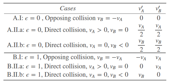
Setting values for $v_A,v_B$, three cases for testing are identified and are repeated for $\epsilon=0,1$. This was a good opportunity to use the Solve function:
(* impulse J *)
j[va_, vb_, r_] := -(1 + r) (va - vb)/2;

(* post-collision velcities *)
eqn = {
   vaP == j[va, vb, r] + va,
   vbP == (-j[va, vb, r]) + vb
   };

(* solve for.. *)
sol = {vaP, vbP};

casesDesc = {
   "A.I: \[Epsilon]=0, Opposing collision, vb \[Equal] -va",
   "B.I: \[Epsilon]=1, Opposing collision, vb \[Equal] -va",
   "A.II.a: \[Epsilon]=0, Direct collision, va>0, vb=0",
   "B.II.a: \[Epsilon]=1, Direct collision, va>0, vb=0",
   "A.II.b: \[Epsilon]=0, Direct collision, va=0, vb<0",
   "B.II.b: \[Epsilon]=1, Direct collision, va=0, vb<0"
   };
cases = {
    {vb -> -va, r -> #},
    {vb -> 0, r -> #},
    {va -> 0, r -> #}
    } &;

sub = {vaP -> "\!\(\*SubscriptBox[\(V\), \(A\)]\)'",
   vbP -> "\!\(\*SubscriptBox[\(V\), \(B\)]\)'",
   vb -> "\!\(\*SubscriptBox[\(V\), \(B\)]\)",
   va -> "\!\(\*SubscriptBox[\(V\), \(A\)]\)"};

TableForm[#[[All, All, 2]],
   TableHeadings -> {casesDesc, #[[1, All, 1]]},
   TableSpacing -> {5, 3}] &[
 Flatten[Table[
    Solve[eqn, sol] /. cases[j][[i]], {i, 1, 3}, {j, 0, 1}], 2] /.
  sub]
The table describes the outcome for the three cases, each evaluated for $\epsilon = 0$ and $1$ and in terms of the final speeds after collision. It makes physical sense as we'd expect bodies to exchange their speeds after an elastic collision or move off together as a single body in the case of a completely inelastic collision.
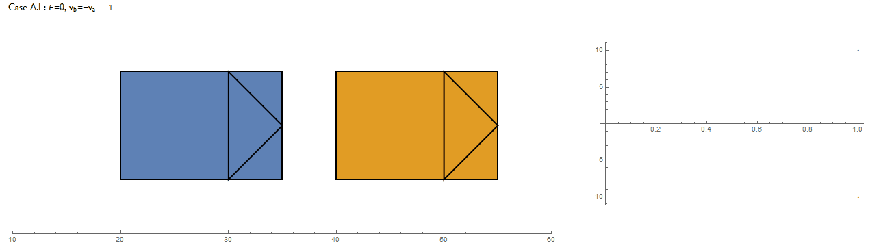
Does the algorithm correctly implement it though? Non-zero speeds are set to $\pm 10$ and $v_A', v_B' $ are the speeds after collision for the blue and orange vehicles respectively. The following shows all 6 cases along with a plot of vehicle speeds against time. Indeed, its a success.
Additional tests:
3-body elastic collision 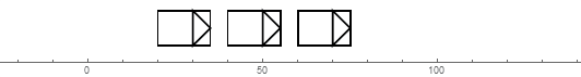
And more.. 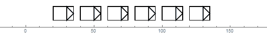
And finally 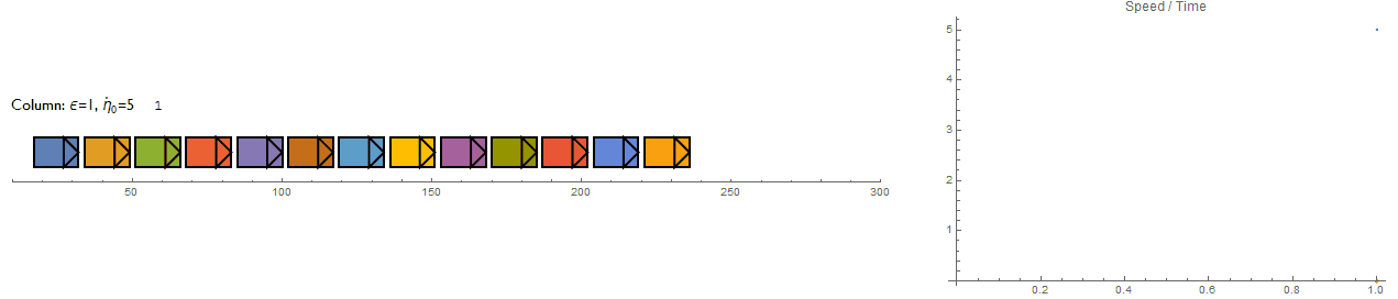
Adding Forces
Calculating vehicle trajectories begins with an acceleration term which incorporates friction and restorative forces. Adding friction was always intended but the inclusion of a spring constant which imparts an acceleration directing the driver towards its initial position was an experiment for fun.
a = -(f*v0) - k (x0 - testConditions[[testID, 1, 1]]);
It worked so I decided to keep it. 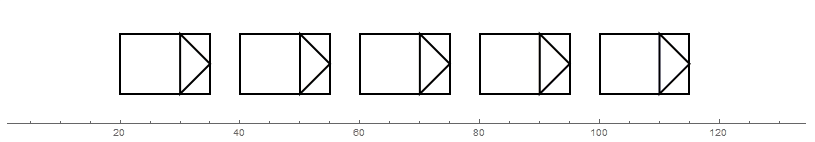
But watching this got me thinking and so I began to focus my attention away from simulating collisions and back to traffic modelling.
Traffic Modelling - The Adventure Continues
Recovering a Macroscopic Model
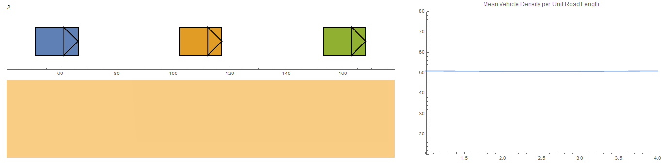
It would be nice to have the option to visualize the flow of individual vehicles (microscopic view) using a heat map (macroscopic view). The concept is illustrated below.
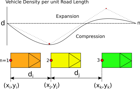
The vehicles are initially equidistant from each other so the initial uniform density represents the baseline to which changes are shown against. The plot of the density curve is achieved via ListLinePlot with an interpolation term added. The heat map is a ListDensityPlot where the plot range is dynamically updated to show slices for a time T. Boundary conditions are imposed via inserting the initial equidistance values at the 'start' and 'end' of the data. The whole lot is wrapped in Manipulate to view it through time.
ListDensityPlot[
   Table[Insert[Differences[testConditions[[All, 1, i]]],
     15 + \[Delta] + \[Sigma] + \[CapitalSigma], {{1}, {-1}}], {i, 1,
     Length[timeList], 1}],
   PlotRange -> {{1, testNum + 1}, {T, T + 1}},
   AspectRatio -> 1/10,
   Axes -> False,
   Frame -> False,
   ImageSize -> 800]

  ListLinePlot[
   Insert[Differences[testConditions[[All, 1, T]]],
    15 + \[Delta] + \[Sigma] + \[CapitalSigma], {{1}, {-1}}],
   PlotRange -> {{1, testNum + 1}, {10, 60}},
   InterpolationOrder -> 2,
   ImageSize -> 500,
   PlotLabel -> "Mean Vehicle Density per Unit Road Length",
   AxesOrigin -> {0, 15 + \[Delta] + \[Sigma] + \[CapitalSigma]}
   ]
I was very pleased with this result, even though the plot is technically upside down. But I was keen to move on..
Experimenting
The mini project was beginning to grow into something much larger so I decided to make it into a standalone model with its own user interface. The UI received quite a bit of attention since having one promotes quick prototyping of different setups but it was also a test bed for various experimental features which I plan to recycle into other projects too (Mathematica Minesweeper is in the queue).
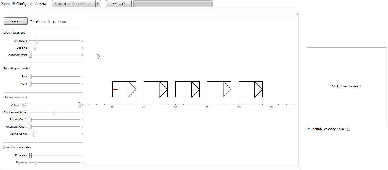
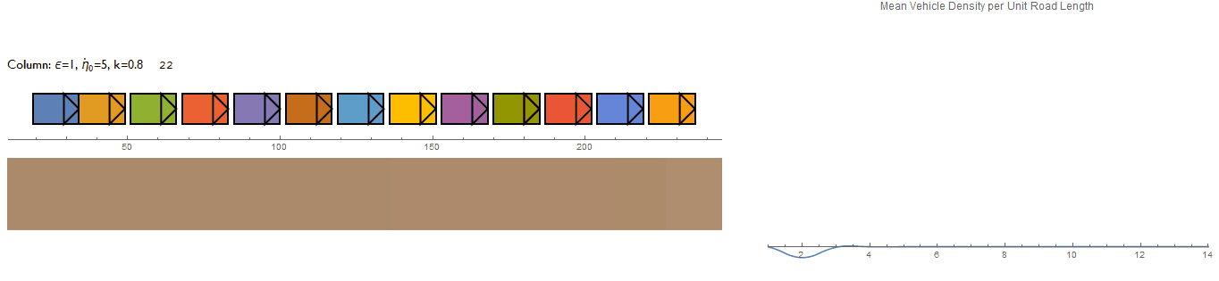
The frame rate has been adjusted to shorten the evaluation time and to compensate for lag when displaying the macroscopic heat map. Also, when setting negative perturbations, the indicator arrows may fail to draw (but the data has been updated - evaluating $\eta$Set will confirm). Also "pertubation" is spelt incorrectly and it should be $\dot{\eta_i}$ instead. But the errors remain since I wanted to move onwards with the project.
The option to increase the bounding box width gives separate control over the front (yellow region) and rear (blue region) values ( $\sigma$ and $\Sigma$ respectively).
Recreating Traffic Density Waves
A phenomena observed in moving traffic, traffic density waves emerge spontaneously as a result of random and subtle shifts in speed by drivers which may induce a sudden deceleration by a following vehicle, which in turn manifests the same response in other drivers further along a column of traffic. The result is a cluster of slow moving vehicles forming a traffic jam - or regions of higher vehicle densities. As this effect propagates down the column, the localized density region appears to move with the properties of a non dispersing wave (soliton).
I've attempted to describe single lane traffic in terms of a system of collisions with oscillatory behaviours:
Values of $\epsilon >1$ represent an over-compensation of speed adjustment for drivers in response to oncoming vehicles. If drivers move within regions defined by $\delta$ then they wont incur any interactions, conversely, approaches sufficient to make contact with the bounding boxes represent a proximity close enough to warrant interaction mediated by elastic collisions. Hence, the approaching driver slows down and the approached driver speeds up.
This is the results from a first attempt where the system receives an initial perturbation by the driver at the left end of the column. The density plot even picks up the soliton traveling through the traffic column. The system's behaviour doesn't appear to be very realistic though.
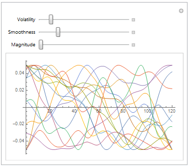
Simulating Random Perturbations
This is an improved approach from an earlier attempt at adding noise into vehicle accelerations.
\[Zeta] =
  (Rescale[
       GaussianFilter[
        RandomFunction[
         WienerProcess[(*drift 0*)#1,(*volatility 0.0001*)#2], \ {0,(*tMax*)#5,(*dt*)#6},(*testNum*)#7],
(* smoothness 200*)#3]] -  0.5)*(* magnitude 60 *)#4 &;

noise = \[Zeta][0, volatility, smoothness, magnitude, tMax, dt, testNum];

noise["SliceData", t][[testID]]
Its a time and state continuous random process generated via a Wiener process which has been smoothed out and rescaled according to parameters set by the user. The noise function is then sliced at discrete points in time during evaluation and added to the drivers initial speed.
The model was now evaluated without any predefined initial perturbations - only random noise is present.
Some of the behaviours aren't quite believable, especially around the boundary vehicles. But there does seem to be an apparent drift of densities visible by the heat map.
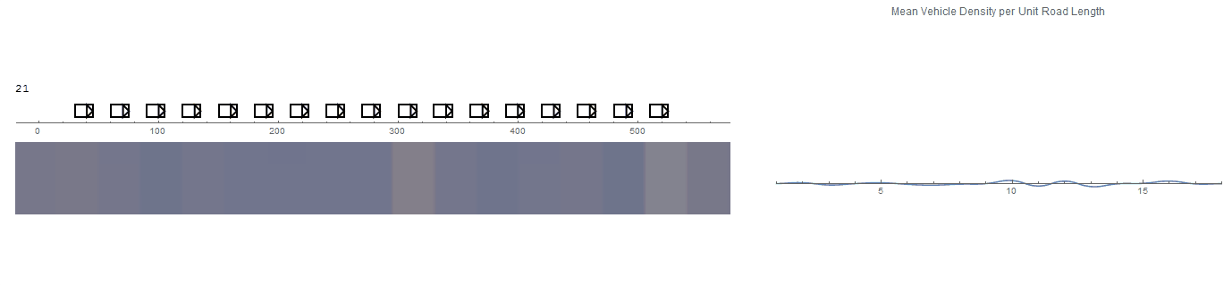
A more believable system is achieved after some adjustments to the model's parameters. The simulation defaults are set to those which gave this result.
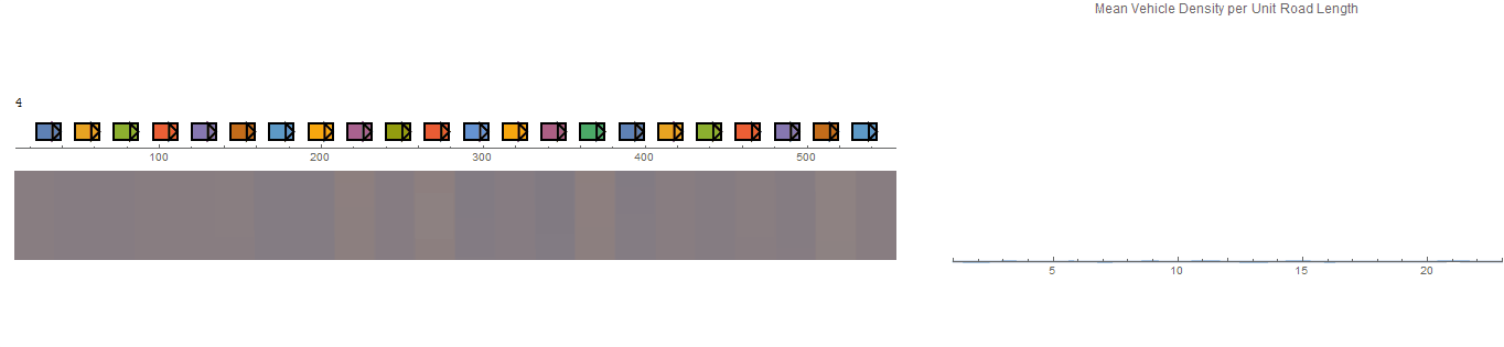
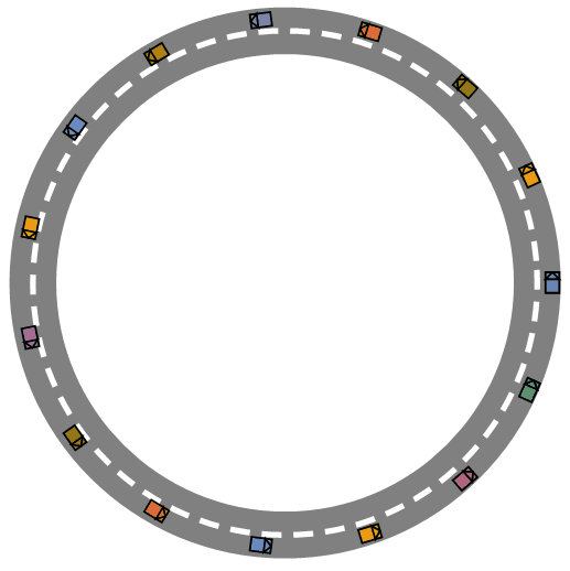
This is the result of using EDI to replicate an experiment conducted by Sugiyama et. al in Traffic jams without bottlenecksexperimental evidence for the physical mechanism of the formation of a jam - and the video can be seen on youtube.
Unfortunately, the results of this experiment (above) fail to demonstrate a travelling density wave as the system appears to reach a steady state, but does show an emergence of queuing due to car-following behaviours. Interestingly, the same vehicle grouping effect can be seen in the collision-based model but with a dynamic characteristic as groups fall in and out of formation.
In the course of this project I've identified a number of avenues for improvement, including implementing the improved noise functionality and repeating the traffic circle experiment. And while the core functionality of EDI works, a complete, stable, verified and calibrated build is still about a month or two away. But a complete description will be posted eventually.
 Attachments:


