Since very early on Stephen Wolfram was interested in how simple rules can lead to very complex behaviour and that interest has obviously not ceased until today. I will look into a couple of very simple examples that would be described as chaotic, stochastic systems and cellular automata and the relationships between them.
I will show how we can use stochastic processes that are related to chaotic systems to generate images just like this:
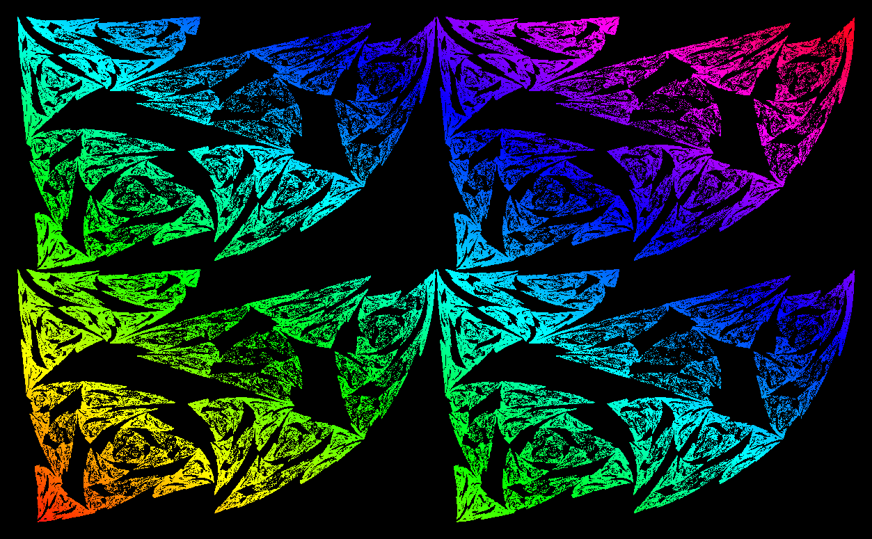
which I think could easily go on one of Sheldon's T-shirt on the @bigbangtheory.
Chaotic Systems
Let's start with a simple chaotic system. It is probably one of the simplest of all chaotic systems: the Bernoulli shift map.
HoldForm[Subscript[x, n + 1] = Mod[2 Subscript[x, n], 1]] // TraditionalForm

It is a really simple rule. Start with a real (normal) number between 0 and 1, multiply the last value by 2 and make sure that the digit on the left of the point is zero. We can easily plot this in Mathematica.
NestList[Mod[2 #, 1] &, 1/Sqrt[2], 100] // ListLinePlot
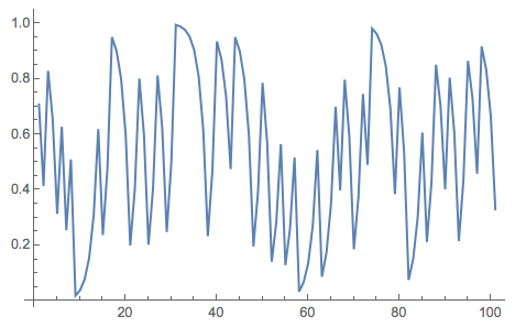
It looks quite erratic, but it is actually deterministic. Given the initial value and iterating a deterministic rule you can compute all the future of the system. The structure behind this simple process can be visualised using a scatterplot:
ListPlot[Partition[NestList[Mod[2 #, 1] &, 1/Sqrt[2], 300], 2, 1]]
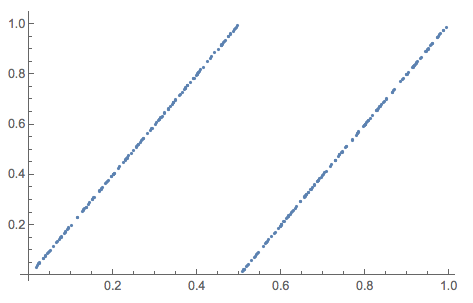
This is actually the function on the right hand side of our recurrence relation:
Plot[Mod[2 x, 1], {x, 0, 1}]
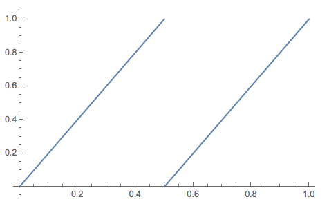
The scatterplot illustrates the simple rule behind this iteration. Which is deterministic. We can also observe that this map is very sensitive to its initial conditions.
\[Delta] = 10^-10;
{NestList[Mod[2 #, 1] &, 1/Sqrt[2], 60], NestList[Mod[2 #, 1] &, 1/Sqrt[2] + \[Delta], 60]} // ListLinePlot
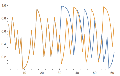
This shows that even if the initial conditions are only off by $10^{-10}$ after about 20 steps the paths diverge and behave very differently. This is of course all known; Ed Lorenz used the term "butterfly effect" for this kind of thing. You will have noticed that I used a very strange unusual intitial condition $1/\sqrt{2}$. This has a reason. It turns out that you need to start at what is called a "normal number".


This basically means that you have to start at a number, the digits of which are generated randomly - a random initial condition. If you started at a finite precision number (like machine precision), i.e. a number where after a finite number of digits there are only zeros, then this function would stop behaving erratically but rather go to a constant zero:
NestList[Mod[2 #, 1] &, RandomReal[], 100] // ListLinePlot
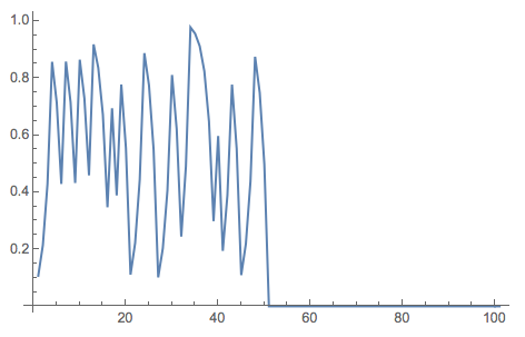
A similar problem happens when you start at numbers with a periodic (binary/decimal) expansion.
NestList[Mod[2 #, 1] &, 1/3, 100] // ListLinePlot
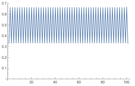
Now the time series is periodic. Neither situation (fixed point or periodic) are typical in the sense that if you randomly pick an initial condition, you obtain a chaotic sequence with probability one. Normal numbers have measure one; typically you would pick a normal number, which is problematic when using many programming languages naivly.
This is a nightmare for simulations of some chaotic systems, as you cannot really generate long time series, because of finite precision. As you see above there is no such problem in Mathemtica when you calculate with infinite precision, i.e. when I use $1/\sqrt{2}$. Of course, I can overcome the problem in the last figure by just increasing the precision:
NestList[Mod[2 #, 1] &, RandomReal[1, WorkingPrecision -> 150], 100] // ListLinePlot
As long as the working precision is a bit larger than the number of iterations the time series will be correct. It is interesting to note that on many machines this problem does not actually present it self (at least not for reasonably long time series). If you program this in C/C++ you can usually do many more iterations then what correponds to the MachinePrecision. This is because the processor " effectively adds" random last digits as you iterate - this is not a very good description, but should suffice for now. In that particular case it actually helps. There is a famous shadowing lemma which allows to conclude that the so generated time series is [Delta] close to a "proper" time series with infinite precision.
One further observation is that the Bernoulli shift map becomes really simple in base 2. This is because in base two multiplication by 2 only shifts all digits one to the left - just like multiplication by 10 in base 10.
TableForm[BaseForm[#, 2] & /@ NestList[Mod[2 #, 1] &, RandomReal[1, WorkingPrecision -> 10], 40]]
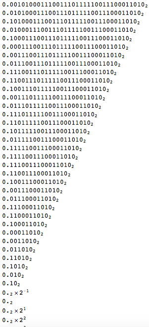
The first line corresponds to our (finite) precision intinial condition. Then we iterate and as you can see the sequence is shifted to the left and any potential nonzero digit on the left of the point is deleted. You also notice that after a certain number of iterations the hole thing goes numerically to zero.
This shifting behaviour in base 2 will become important now.
Stochastic systems with time reversal
Let's give the story a nice twist. The idea is taken from this paper; for a very readable description see here. In the section on chaos we had a deterministic system with random initial conditions. Let's go to a stochastic system like so:
HoldForm[Subscript[x, n + 1] = 1/2 Subscript[x, n] + 1/2 RandomChoice[{1, 2}]] // TraditionalForm

This system would usually be considered to be stochastic. Its dynamics is mainly determined by previous values plus noise similar to ARProcesses. The curious thing is that if I time reverse the resulting time series, the system becomes identical to the chaotic system in part one!
ListLinePlot[Reverse@NestList[1/2 # + 1/2 RandomChoice[{0, 1}] &, RandomReal[], 40]]
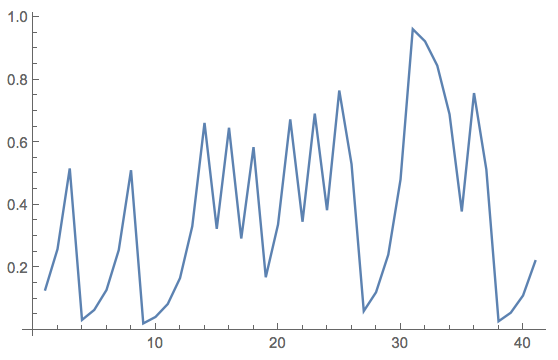
This time series does not fully make my point so let me be a bit clearer. First we choose an initial condition (and try to be a bit generous about the number of digits):
start = RandomReal[1, WorkingPrecision -> 400];
Then we generate our time series and plot:
tsdeterm = NestList[Mod[2 #, 1] &, start, 100];
ListLinePlot[tsdeterm]
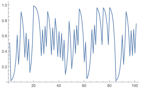
Now comes the trick. I use the 100th value of the time series, and convert it to binary (after padding it on the left with zeros). Then I extract the individual digits:
randomincrements =
 Join[ConstantArray[0, -RealDigits[tsdeterm[[-100]], 2][[2]]], RealDigits[tsdeterm[[-100]], 2][[1]]];
Finally, I use my stochastic system with these random increments:
results = {tsdeterm[[-1]]}; Do[AppendTo[results, 1/2 results[[-1]] + 1/2 randomincrements[[100 - i]]], {i, 1, 100}]
Then I reverse the time series and plot it with the original, deterministic one:
ListLinePlot[{tsdeterm[[1 ;;]], Reverse@results}, PlotStyle -> {{Red, Thick}, {Blue, Dotted}}]
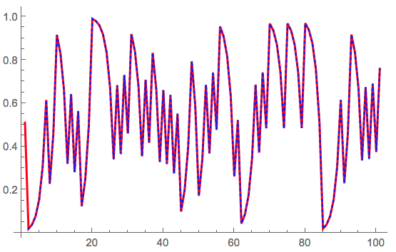
It becomes clear that the two sequences are identical - well at least for long enough random sequences. So basically I used the values of the deterministic sequence (in binary form) as increments of my stochastic time series and get the same result - after time reversal. So my random initial condition acts as "random increments" in my stochastic system and makes them - sort of- equivalent. We can look at the scatter plots of both and they are, of course, identical:
Row[
{ListPlot[Partition[tsdeterm, 2, 1], PlotStyle -> Green, ImageSize -> Medium],
ListPlot[Partition[Reverse@results, 2, 1], PlotStyle -> Red, ImageSize -> Medium]}]

Alternatively and probably easier, I could first generate the random increments and then the corresponding initial condition for the deterministic system. If we generate the (chaotic) time series like this we do not have to care -very much- about the finite precision of the computer arithmetic, which is a huge advantage.
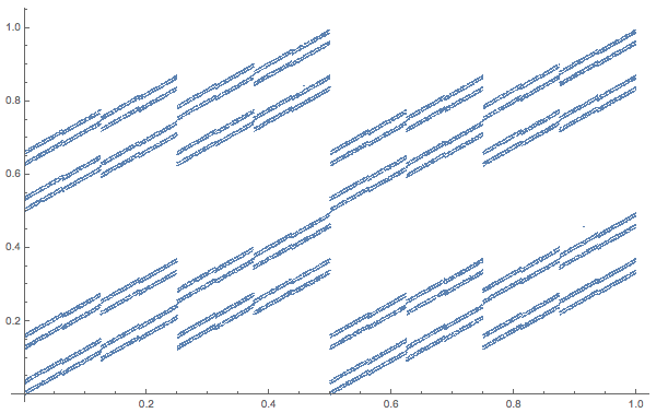
We can now also combine two of these stochastic equations and get some interesting structures - the only really important thing seems to be that the random increments are "very discrete", i.e. that there are only few possible values.
ListPlot[Reverse@
  NestList[{1/2 #[[1]] + 1/2 RandomChoice[{0, 1}], 1/4 #[[2]] + 1/4 #[[1]] + 1/2 RandomChoice[{0, 1}]} &, RandomReal[1, 2], 45000], PlotMarkers -> {Point, 0.1}]
Or this one:
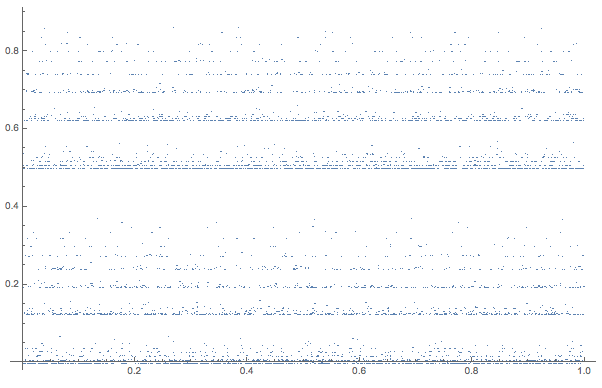
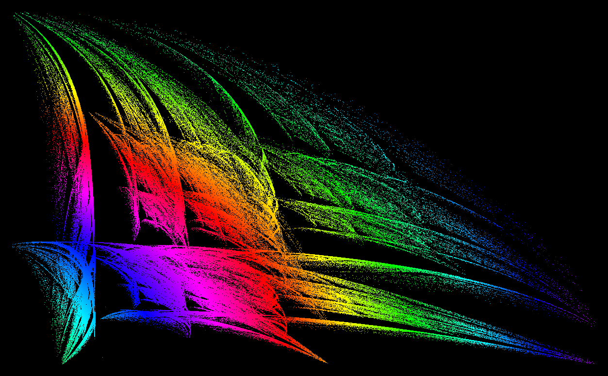
By playing a bit with the functional form of the equations we can achieve some pretty results:
Brushstrokes
databrushstrokes =
  Reverse@NestList[{1/2 Cos[-0.3 (#[[1]]^2 + #[[2]]^2)] + 1/2 RandomChoice[{0, 1, 2}] #[[2]],
      1/2 Sin[#[[1]]]*Cos[#[[2]]] + 1/2 RandomChoice[{0, 1}] #[[1]]} &, RandomReal[1, 2], 1000000];
Graphics[{PointSize[0.0005], Point[databrushstrokes, VertexColors -> (Hue /@ (Norm[#] & /@ brushstrokes))]},
 AspectRatio -> 1/GoldenRatio, Axes -> False, Background -> Black, Axes -> False, ImageSize -> Full]
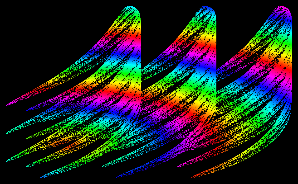
Three ghosts
datathreeghosts =
  Reverse@NestList[{1/2 Cos[-0.3 (#[[1]]^2 + #[[2]]^2)] + 1/2 RandomChoice[{0, 1, 2}],
      1/2 Sin[#[[1]]] + Cos[#[[2]]] + 1/2 RandomChoice[{0, 1, 2}]} &, RandomReal[1, 2], 1000000];
Graphics[{PointSize[0.0005], Point[datathreeghosts, VertexColors -> (Hue /@ (Norm[#] & /@ datathreeghosts))]},
 AspectRatio -> 1/GoldenRatio, Axes -> False, Background -> Black, Axes -> False, ImageSize -> Full]
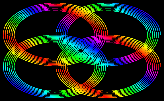
Olympic Rings
dataolympicrings =
  Reverse@NestList[{1/2 Cos[10 Pi*(#[[1]]^2 + #[[2]]^2)]*Exp[-0.2*(#[[1]]^2 + #[[2]]^2)] + 1/2 RandomChoice[{0, 1}],
      1/2 Sin[10 Pi*(#[[1]]^2 + #[[2]]^2)]*Exp[-0.2*(#[[1]]^2 + #[[2]]^2)] + 1/2 RandomChoice[{0, 1}]} &, RandomReal[1, 2], 600000];
Graphics[{PointSize[0.002], Point[dataolympicrings, VertexColors -> (Hue /@ (Norm[#[[1]] + #[[2]]] & /@
 dataolympicrings))]}, AspectRatio -> 1/GoldenRatio, Axes -> False, Background -> Black, Axes -> False, ImageSize -> Large]
Jellyfish
datajellyfish =
  Reverse@NestList[{1/2 Cos[#[[1]]] + 1/2 Sin[#[[2]]] + 1/2 RandomChoice[{0, 1}] #[[2]],
      1/2 Cos[#[[2]]] + 1/2 Sin[#[[1]]] + 1/2 RandomChoice[{0, 1}] #[[1]]} &, RandomReal[1, 2], 2000000];
Graphics[{PointSize[0.0002], Point[datajellyfish, VertexColors -> (Hue /@ (Norm[#] & /@ datajellyfish))]},
 AspectRatio -> 1, Axes -> False, Background -> Black, Axes -> False, ImageSize -> Full]

FractalMan with hat
datafractalman =
  Reverse@NestList[{1/2 Exp[-3 (#[[1]]^2 + #[[2]]^2)] + 1/2 RandomChoice[{0, 1}],
  1/2 #[[1]]^#[[2]] + 1/2 RandomChoice[{0, 1}]} &, RandomReal[1, 2], 4000000];
Graphics[{PointSize[0.0004], Point[datafractalman, VertexColors -> (Hue /@ Mean /@ datafractalman)]},
 AspectRatio -> 1/GoldenRatio, Axes -> False, Background -> Black, Axes -> False, ImageSize -> Full]

If you just look at the time series everything looks very weird and erratic. Here are the two sequences for the olympic rings:
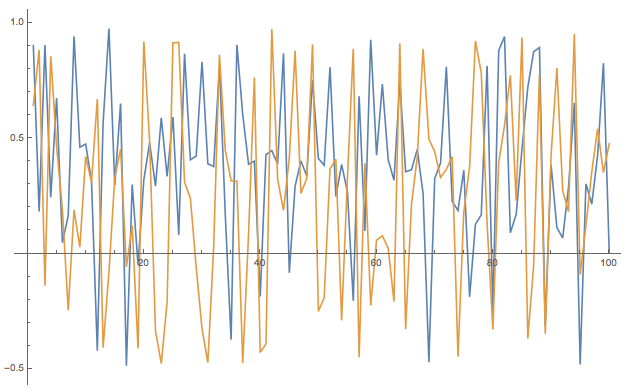
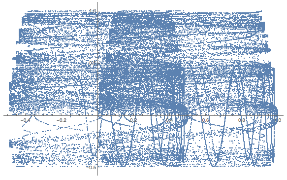
and here their scatterplot:
ListPlot[Partition[dataolympicrings[[1 ;;, 1]], 2, 1]]
Further examples
Here are some more examples for you to try:
datamesh =
  Reverse@NestList[{1/2 Cos[10 Pi*(#[[1]]^2 + #[[2]]^2)]*
        Exp[-0.2*(#[[1]]^2 + #[[2]]^2)] + 1/2 RandomChoice[{0, 1}],
      1/2 SawtoothWave[10 Pi*(#[[1]]^2 + #[[2]]^2)]*
        Exp[-0.2*(#[[1]]^2 + #[[2]]^2)] + 1/2 RandomChoice[{0, 1}]} &,
     RandomReal[1, 2], 60000];
Graphics[{PointSize[0.002],
  Point[datamesh,
   VertexColors -> (Hue /@ (Norm[#[[1]] + #[[2]]] & /@ datammesh))]},
 AspectRatio -> 1/GoldenRatio, Axes -> False, Background -> Black,
 Axes -> False, ImageSize -> Large]
datasqueezedrings =
  Reverse@NestList[{1/2 SawtoothWave@Sin[10 Pi*(#[[1]]^2 + #[[2]]^2)]*
        Exp[-0.2*(#[[1]]^2 + #[[2]]^2)] + 1/2 RandomChoice[{0, 1}],
      1/2 SawtoothWave@Cos[10 Pi*(#[[1]]^2 + #[[2]]^2)]*
        Exp[-0.2*(#[[1]]^2 + #[[2]]^2)] + 1/2 RandomChoice[{0, 1}]} &,
     RandomReal[1, 2], 100000];
Graphics[{PointSize[0.002],
  Point[datasqueezedrings,
   VertexColors -> (Hue /@ (Norm[#[[1]] + #[[2]]] & /@
        datasqueezedrings))]}, AspectRatio -> 1/GoldenRatio,
 Axes -> False, Background -> Black, Axes -> False, ImageSize -> Large]
dataflowers =
  Reverse@NestList[{1/10 (#[[1]]^2 + #[[2]]^2) +
       1/2 RandomChoice[{0, 1, 2}],
      1/3 (Sin[#[[1]]] + Cos[#[[2]]]) +
       1/2 RandomChoice[{0, 1, 2}]} &, RandomReal[1, 2], 20000];
Graphics[{PointSize[0.002],
  Point[dataflowers,
   VertexColors -> (Hue /@ (Norm[#[[1]] + #[[2]]] & /@
        dataflowers))]}, AspectRatio -> 1/GoldenRatio, Axes -> False,
 Background -> Black, Axes -> False, ImageSize -> Large]
These coupled stochastic maps seem to be fractal generators! Ususally fractals are linked to chaotic systems, but there are some exceptions.
Stochastic Sierpinski Triangle
The Sierpinski triangle is a fractal object. You start with a triangle remove a little triangle in the middle and iterate. This is a very deterministic procedure which yields a fractal object. See this demonstration.
It turns out that the same object can be generated by a stochastic procedure: 1. choose a random point in the plane. 2. Construct a triangle; label the three vertices of the first triangle by 1,2,3. 3. Chose a vertex at random and move half way towards it. 4. Iterate step 3.
Here is an implementation of that.
M = 40000;
randompoints = Table[RandomChoice[{{0., 0.}, {1., 0.}, {0.5, Sqrt[3]/2 // N}}], {i, 1, M}]; results = {RandomReal[1, {2}]}; Table[
 AppendTo[results, 0.5*(randompoints[[i]] - results[[-1]]) + results[[-1]]], {i, 1, M}];
ListPlot[results, ImageSize -> Large, AspectRatio -> 1, Axes -> False]
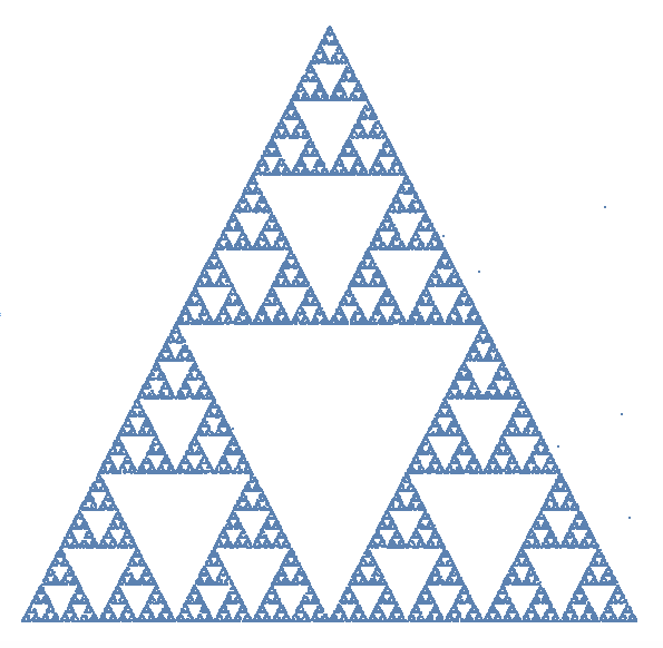
It turns out that this is only one of our stochastic systems with discrete but dependent increments:
data = NestList[
    1/2 ({ 1 #[[1]], #[[2]]} + RandomChoice[{{0., 0.}, {1, 0.}, {0.5, Sqrt[3]/2 // N}}]) &, RandomReal[1, 2], 100000][[5 ;;]];
Graphics[{PointSize[0.0002], Yellow, Point[data(*,VertexColors\[Rule](Hue/@Mean/@data)*)]},
 AspectRatio -> 1/GoldenRatio, Axes -> False, Background -> Black, Axes -> False, ImageSize -> Full]
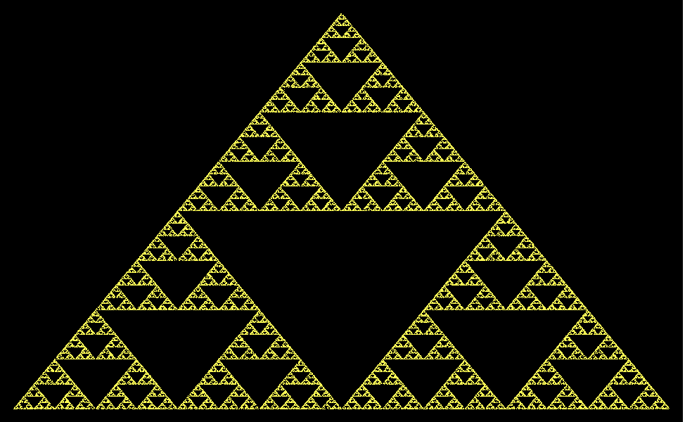
You can now deform this a bit and try things like this:
data = NestList[
    1/2 ({ #[[1]], #[[2]]^1.3} +
        RandomChoice[{{0., 0.}, {1., 0.}, {0.5, Sqrt[3]/2 // N}}]) &,
    RandomReal[1, 2], 100000][[5 ;;]];
Graphics[{PointSize[0.0002], Yellow,
  Point[data(*,VertexColors\[Rule](Hue/@Mean/@data)*)]},
 AspectRatio -> 1/GoldenRatio, Axes -> False, Background -> Black,
 Axes -> False, ImageSize -> Full]
Cellular Automata
Finally, it has repeatedly been observed that cellular automata can also produce chaotic signals. We might therefore want to figure out which cellular automaton corresponds roughly to the Bernoulli Shift Map. We work in binary representation:
CellularAutomaton[170, RandomChoice[{0, 1}, 12], 6] // TableForm

So similar to the Bernoulli Shift Map rule 170 shifts the sequence one step to the left. This means that we can now generate the Bernoulli Shift map with that rule:
N[FromDigits[{#, 0}, 2]] & /@ CellularAutomaton[170, RandomChoice[{0, 1}, 300], 250] // ListLinePlot
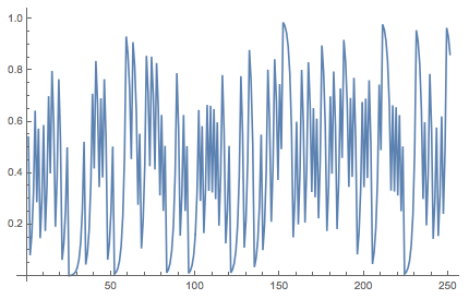
If we look at the scatterplot we can corroborate the typical pattern of the Bernoulli shift map:
ListPlot[Partition[N[FromDigits[{#, 0}, 2]] & /@ CellularAutomaton[170, RandomChoice[{0, 1}, 1000], 950], 2, 1]]
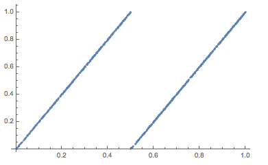
We can now put two of them together to get a two dimensional system.
ts = {{RandomChoice[{0, 1}, 100], RandomChoice[{0, 1}, 100]}};
Do[AppendTo[ts, {CellularAutomaton[170, ts[[-1, 1]], 1][[2]], CellularAutomaton[170, ts[[-1, 2]], 1][[2]]}], {80}];
ListPlot[{N[FromDigits[{#[[1]], 0}, 2]], N[FromDigits[{#[[2]], 0}, 2]]} & /@ ts]
This is neither fast not elegant but does the job. If we now couple the two equations, but converting to decimal, applying some functions and converting back to binary
ts = {{RandomChoice[{0, 1}, 40000], RandomChoice[{0, 1}, 40000]}};
Do[AppendTo[ts, {Join[ConstantArray[0, -RealDigits[#, 2][[2]]],
       RealDigits[#, 2][[1]]] & @(Sin[1.8*N[FromDigits[{CellularAutomaton[170, ts[[-1, 1]], 1][[2]], 0}, 2]] +
        N[FromDigits[{CellularAutomaton[170, ts[[-1, 2]], 1][[2]], 0},2]]]), Join[ConstantArray[0, -RealDigits[#, 2][[2]]],
       RealDigits[#, 2][[1]]] & @(1/2 ( N[FromDigits[{CellularAutomaton[170, ts[[-1, 1]], 1][[2]], 0},2]]^3 +
         N[FromDigits[{CellularAutomaton[170, ts[[-1, 2]], 1][[2]], 0}, 2]]^3.))}], {39900}];
ListPlot[{N[FromDigits[{#[[1]], 0}, 2]], N[FromDigits[{#[[2]], 0}, 2]]} & /@ ts, Axes -> False,
 Background -> Black, PlotStyle -> Yellow, PlotMarkers -> {Point, 0.1}]
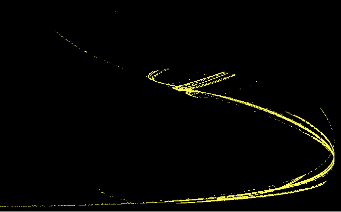
There is nothing really new here, but we do generate some nice images. Many other ideas come to mind, but this post is already much too long, so I will call it a day.
Cheers,
Marco