Introduction
My last post was eventually concerned with finding the shortest path through a maze and potential applications to a separate project on simulating urban traffic. The solution to solving the maze was ultimately found by flooding it not very realistic but it did so without prior knowledge of the mazes layout. So as a response to this and also to research more methods in pathfinding and obstacle avoidance, Ive written an agent who can navigate a maze (or arbitrary environment of obstacles). It aims to display realistic behaviours and capabilities when exploring. Its goal is to escape by reaching any point on the boundary of its environment and does so by exploring; walking towards unseen territory. The program is presented with a user interface to easily draw mazes, monitor progress and review the agents daring escape.
Calculating Field of View (FOV)
The user draws obstacles by setting points for B Spline curves. Coordinates which lie on the curves are detected within the agents FOV and interpreted as obstructions (walls).
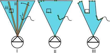
Fig. 1. (I) Agent scans for obstacles. (II) Intersection between scanning region and environment produce points. (III) Points form FOV region.
The region search is defined as a rectangle plotted from the agent's origin to the length of it's sight range (range) and takes an argument for angle of rotation which is picked from the list scan.
search = TransformedRegion[
    Rectangle[{#1 + #6, #2 - 0.2}, {#1 + #6 + #3, #2 + 0.2}],
    RotationTransform[#5, {#1, #2}]] &;

scan = Range[-\[Phi]/2, \[Phi]/2, 0.01];
Region membership determines if any points (representing obstructions) in the environment fall within search (Fig 1. i). If so, the point is appended to a list. For the case of more than one point (Fig 1. iii), then the point nearest to the agent's origin is returned. If no points are detected (Fig 1. ii) then a point is calculated according to the length range at a rotation of the current scan value.
AngleVector[{pt[[1]], pt[[2]]}, {range + scale, \[Theta] + scan[[i]]}]
Once complete, the scanning angle is incremented by picking the next value from scan and the process is repeated until the last element from scan has been picked.
(* determine FOV region *)
FOVcalc := (
   (* inc. steps *)
   scan = Range[-\[Phi]/2, \[Phi]/2, 0.01];
   (* `viewlist` keeps list of XY points used to draw polygon,
   represented as region *)

   (* flags list elements representing walls "W" or limit of sight \
"L" *)
   viewList = ReplacePart[#,
       Normal[
        AssociationThread[
         Position[Total /@ Map[Length, #, {2}],
           0] -> (Insert[#, "W", -1] & /@
            Partition[
             Extract[#, Position[Total /@ Map[Length, #, {2}], 0]],
             1])]
        ]
       ] &[Insert[Table[
       (* while scanning, if no obstruction is detected,
       return maximal point,
       if obstruction is detected and there exists more than one \
point, return point closest to origin (agent location), else,
       return detected point *)
       If[Length[Dimensions[#]] > 1,
          Keys[TakeSmallest[<|
                Thread[# ->
                    EuclideanDistance[#, {pt[[1]], pt[[2]]}] & /@ #]|>,
                1]][[1]] &[#], #] &[
        Extract[Flatten[map, 1],

          Position[
           RegionMember[
             search[pt[[1]], pt[[2]],
              range, \[Phi], \[Theta] + scan[[i]], scale]][
            Flatten[map, 1]], True]] /.
         x_ /; x == {} -> {AngleVector[{pt[[1]],
             pt[[2]]}, {range + scale, \[Theta] + scan[[i]]}],
           "L"}], {i, 1, Length[scan]}], {pt[[1]], pt[[2]]}, 1]
     ]
   );
Ultimately, evaluating FOVcalc generates the list of points viewList which are used to draw a polygon as the basis for the FOV region (Fig. 1 iii).
The attached notebook contains cells for producing such demonstrations as below: 
Its noted that altering the default sight angle raises some scaling issues.
Generating the Virtual Environment
Agent evaluates rotateSearch
(* calculates new FOV, enviroment data and traversal graph *)
look := (
   FOVcalc; refreshAgentVision; computeGraphSpace;
   AppendTo[sessionData, {Values[env], pMap}]
   );

(* agent looks while performing full rotation *)
rotateSearch := Do[
   \[Theta] += \[Pi]/4;
   look,
   8
   ];
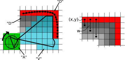
Discretized spline functions give a list of coordinates which are employed via FOVcalc to return the location of walls ("O"). Region membership between newly calculated FOV region and environment coordinates return space which is currently visible ("V") while yielding space which was previously visible and thus discovered ("D"). Member coordinates of the agent's footprint are set as "A". The distance from each discovered or visible coordinate to the nearest wall coordinate is calculated and used to weigh further computations.
Equipped with an agent which can see, we now use this to define where obstacles lie within the FOV and ultimately return information of what the perceived environment looks like. First, we get the location of obstacles (walls).
walls := DeleteDuplicates[
   IntegerPart /@
    Rest[Extract[viewList, Position[viewList, {_, "W"}]][[All, 1]]]];
Entries in viewList are flagged with either a "W" (wall) or "L" (limit of sight) so extracting the correct entries is easy. If we didn't make the classification then points generated at the limit of the sight range would be interpreted as walls.
The perceived environment is stored as an array of characters with dimensions equal to the width (xLen) and height (yLen) of the environment (default 100x100).
env = AssociationThread[Flatten[Array[{#1, #2} &, {xLen, yLen}], 1],
   ConstantArray["E", xLen*yLen]];
Initially constant ("E" for empty), entries are updated as the agent sees more of it's surroundings. For example,
(* draw walls *)
Do[(env[#[[i]]] = "O"), {i, 1, Length[#]}] &[walls];
Since the environment array is used to review the programs output, we also add other useful information such as the agent's current position
(* highlight agent position *)
Do[(env[#[[i]]] = "A"), {i, 1, Length[#]}] &[
  Complement[
   Position[
    ArrayReshape[
     RegionMember[Disk[{pt[[1]], pt[[2]]}, scale], Keys[env]], {xLen,
      yLen}], True]
   , walls]
  ];
and it's FOV
(* highlight current FOV *)
Do[(env[#[[i]]] = "V"), {i, 1, Length[#]}] &[
  Keys[KeyTake[env,
    Position[
     ArrayReshape[
      RegionMember[Polygon[viewList[[All, 1]]]][Keys[env]], {xLen,
       yLen}], True]]]];
We want to know the distance each location has to the nearest wall for later computation
(* - calculates to-wall distances for navigation - *)
(* XY cords for visible space and walls *)
visibleSpace = Keys[Select[env, # == "V" &]];
obstructed = Keys[Select[env, # == "O" &]];
(* compute distance to nearest wall for each member of `visibleSpace` \
*)
toWallDistances = Table[
   IntegerPart[
    N[Min[EuclideanDistance[visibleSpace[[i]], #] & /@ obstructed]]]
   , {i, 1, Length[visibleSpace]}];
The to-wall distances for each location are held in the array pMap
(* update to-wall distances for each visible location *)
pMap = ReplacePart[pMap,
   Normal[AssociationThread[visibleSpace -> toWallDistances]]];
Then, for presentation, a colour scheme is defined which translates the to-wall distances into something more intuitive
(* abs. scaled color rules generate gradients using to-wall distances \
*)
colRulesWallDist =
  Join[ReplacePart[
    Normal[AssociationThread[
      Range[0, 15] -> GrayLevel /@ (N@Range[0, 15]/15)]],
    1 -> (0 -> RGBColor[0.4, 0.5, 0.6])],
   Normal[
    AssociationThread[
     Range[16, Max[{xLen, yLen}]] ->
      Table[GrayLevel[1.], Length[Range[16, Max[{xLen, yLen}]]]]]
    ]
   ];
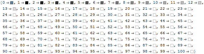
Like env, pMap is also initially constant (0) and its values are procedurally updated. A value of 0 means that this corresponding environment location is undiscovered. As the agent explores, these values will be replaced and the maze begins to emerge.
(* updates visible enviroment *)
refreshAgentVision := (
   (* remove previous agent position (if applicable) *)
   Do[(env[#[[i]]] = "D"), {i, 1, Length[#]}] &[
    Keys[Select[env, # == "A" &]]];

   (* highlight agent position *)
   Do[(env[#[[i]]] = "A"), {i, 1, Length[#]}] &[
    Complement[
     Position[
      ArrayReshape[
       RegionMember[Disk[{pt[[1]], pt[[2]]}, scale],
        Keys[env]], {xLen, yLen}], True]
     , walls]
    ];

   (* ammend previous FOV as 'discovered' (if applicable) *)
   Do[(env[#[[i]]] = "D"), {i, 1, Length[#]}] &[
    Keys[Select[env, # == "V" &]]
    ];

   (* highlight current FOV *)
   Do[(env[#[[i]]] = "V"), {i, 1, Length[#]}] &[
    Keys[KeyTake[env,
      Position[
       ArrayReshape[
        RegionMember[Polygon[viewList[[All, 1]]]][Keys[env]], {xLen,
         yLen}], True]]]];

   (* draw walls *)
   Do[(env[#[[i]]] = "O"), {i, 1, Length[#]}] &[walls];

   (* - calculates to-wall distances for navigation - *)
   (* XY cords for visible space and walls *)
   visibleSpace = Keys[Select[env, # == "V" &]];
   obstructed = Keys[Select[env, # == "O" &]];
   (* compute distance to nearest wall for each member of \
`visibleSpace` *)
   toWallDistances = Table[
     IntegerPart[
      N[Min[EuclideanDistance[visibleSpace[[i]], #] & /@ obstructed]]]
     , {i, 1, Length[visibleSpace]}];

   (* update to-wall distances for each visible location *)
   pMap =
    ReplacePart[pMap,
     Normal[AssociationThread[visibleSpace -> toWallDistances]]];

   (* procedurally scaled color rules generate gradients using to-
   wall distances *)
   (*colRulesWallDist=ReplacePart[Normal[AssociationThread[Range[0,#]->
   GrayLevel/@(N@Range[0,#]/#)]]&[Max[Flatten[pMap]]],1\[Rule](0->
   RGBColor[0.4,0.5,0.6])];*)


   (* abs. scaled color rules generate gradients using to-
   wall distances *)
   colRulesWallDist =
    Join[ReplacePart[
      Normal[AssociationThread[
        Range[0, 15] -> GrayLevel /@ (N@Range[0, 15]/15)]],
      1 -> (0 -> RGBColor[0.4, 0.5, 0.6])],
     Normal[
      AssociationThread[
       Range[16, Max[{xLen, yLen}]] ->
        Table[GrayLevel[1.], Length[Range[16, Max[{xLen, yLen}]]]]]
      ]
     ];
   );
And the corresponding colour scheme
(* draws enviroment according to color rules *)
colRules = {"A" -> Hue[0.3, 0.8, 0.3], "E" -> Hue[0, 0, 0, 0],
   "O" -> Red, "V" -> Hue[0.5, 0.5, 0.75, 0.3],
   "D" -> Hue[0, 0, 0, 0]};

An early implementation of this as an example is below 
Navigating the Environment
The agent cannot be able to walk through walls so coordinates assigned as obstructions are excluded when considering where the agent can move to.
pSpace = Select[env, # == "V" || # == "D" || # == "A" &];
Since the agent's dimensions are also greater than one unit of space, it also cannot occupy regions immediately next to a wall. Thus we use the to-wall distances from earlier to compute a set of invalid space.
(* vertex coordinates *)
vCoords = Keys[pSpace];

vWeigths = Table[Extract[pMap, #[[i]]], {i, 1, Length[#]}] &[vCoords];

(* vertices with to-wall distance greater than scale *)
invSpace = Extract[vCoords, Position[vWeigths, _?(# < scale - 1 &)]];
All together, this forms the basis for traversalGraph; the graph of locations which the agent can potentially travel to.
traversalGraph =
  Graph[Flatten[
    Table[Table[#[[1]] \[DirectedEdge] #[[2, i]], {i, 1,
           Length[#[[2]]]}] &[{#[[j]],
           Intersection[NN[#[[j]]], #]} &[#]], {j, 1, Length[#]}] &[
     Keys[KeyDrop[pSpace, invSpace]]], 1]
   ];
That's not quite enough though as its possible that the agent will see a region of space through a gap too small to travel through but decide to go there anyway. This region may still be valid but unconnected form its current position. There also needs to be a means of choosing a valid point to traverse to and are categorized by needsRotation and needsTraversal (old terminology from much earlier in the project).
These points of traversal are referred to as sight edges, i.e., places the agent can't see and thus would like to travel to.
(* end locations not bordering to-wall limits - i.e., dead-ends.  \
excludes unconnected vertices *)
sightEdges := Intersection[
   ConnectedComponents[traversalGraph, {verticeLocation}][[1]],
   Complement[
    Extract[VertexList[traversalGraph],
     Position[VertexDegree[traversalGraph], _?(# < 8 &)]],
    Extract[vCoords, Position[vWeigths, _?(# < scale &)]]]
   ];
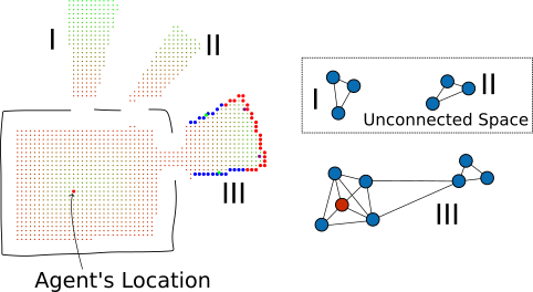
Fig 2. Vertices within section III are all connected to the agent's position, while conversely, I and II are unconnected and so contained points are excluded when returning list of sight edges.
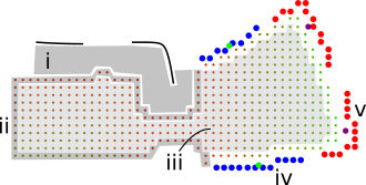
Fig 3. (i) Of all connected space, vertices within the to-wall limit are naturally excluded. (ii) Vertices with degree less than 8 are included except if they neighbour the to-wall limit - travelling there would yield no further discovery. (iii) Interior vertices (degree 8) are excluded since they are not edges. Lastly, what remains are assumed to represent locations to explore (sight edges). Blue points and red points represent needsRotation (iv) and needsTraversal (v) respectively.
(* points bordering uncovered space - select only points neighbouring \
at lest one uncovered location *)

(* points within sight range *)
needsRotation :=
  Keys[Select[
      AssociationThread[# -> (AllTrue[#, # == "D" &] & /@ (Values[
            KeyTake[env, #] & /@ (NN /@ #)]))],
      # == False &]
     ] &[
   Keys[Select[sightEdgeDistances, # <= range &]]
   ];

(* points at limit of sight range *)
needsTravel :=
  Keys[Select[
      AssociationThread[# -> (AllTrue[#, # == "D" &] & /@ (Values[
            KeyTake[env, #] & /@ (NN /@ #)]))],
      # == False &]
     ] &[
   Keys[Select[sightEdgeDistances, # > range &]]
   ];
We've narrowed down the environment to a small list of possible locations to explore, yet many of them are very similar so we can refine this selection even further.
(* clusters and find central location of points *)
clusterCP = Table[{
       Total[First /@ #[[i]]]/Length[First /@ #[[i]]],
       Total[Last /@ #[[i]]]/Length[Last /@ #[[i]]]
       }, {i, 1, Length[#]}] &[FindClusters[#]] &;
Applying clusterCP with any list of sight edges returns the point which is the average location of groups of sight edges. The green and purple points in Fig. 3 are calculated via
Graphics[{
  {PointSize -> Large, Green, Point[clusterCP[needsRotation]]},
  {PointSize -> Large, Purple, Point[clusterCP[needsTravel]]}
}]
Ultimately, the agent will need to decide which of these points (held as a list opt) it should travel to.
(* candidate targets to walk to *)
opt := Flatten[
   Nearest[Keys[KeyDrop[pSpace, invSpace]], #, 1] & /@ Join[
     clusterCP[needsRotation],
     clusterCP[needsTravel]
     ], 1];
Finding an Optimal Path
The agent finds a path between its current position and each of the clustered sight edges.
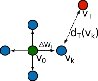
A path between the agents current position ( $v_0$) and target ( $v_T$) which minimizes path length while maximizing to-wall distances is searched for. For the k neighbouring vertices, distance to target ( $d_T(v_k)$) and to-wall gradient ( $ \Delta W_i $) are calculated. Each of the k vertices is assigned a score via
$w_1 d_T(v_k) - w_2 \Delta W $
The chosen vertex is that with the minimal score.
(* searches visible and discovered space for path between v0 and \
target *)
While[v0 != verticeTarget,
 v0 = #[Min[Keys[#]]] &[(*
    looks at NNs to v0 and scores each based on distance to target \
and distance from wall *)
    AssociationThread[
     (w1*vertexDistanceToTarget /@ Complement[moveTo, path] - (w2*
          Lookup[searchSpaceWeigths, Complement[moveTo, path]])) ->
      Complement[moveTo, path]
     ]
    ];
Sometimes this algorithm fails to converge so each path is checked afterwards for convergence to target. If it fails, the path is recomputed under settings favouring a more direct route.
(* checks path - if optimal path could not be found then a more \
direct route is attempted untill one is found *)
While[
  MemberQ[path, Missing["KeyAbsent", \[Infinity]]] == True(*
  path uncomplete *),
  w1 += 1(* shift importance to finding more direct route *);
  If[w1 >= 10, w1 = 1; w2 = 1](* attempts to find most direct path *);
  (* if still not found, abort and return partial path *)
  If[w1 == 9 && w2 == 1, path = Most@path; verticeTarget = path[[-1]];
    Break[]];
  start];
Once a path is returned, it is reduced to its shortest form and smoothed with MovingAverage to appear more natural.
(* reduce solution path to shortest form *)
path = FindShortestPath[
   Graph[
    Flatten[
     Table[
      Table[
         path[[#]] \[DirectedEdge] (NN /@ path)[[#, i]], {i, 1,
          Length[(NN /@ path)[[#]]]}] &[j],
      {j, 1, Length[path]}], 1]
    ], verticeLocation, verticeTarget];

(* smooth path *)
path = Insert[
  Insert[MovingAverage[path, 10], verticeLocation, 1],
  verticeTarget, -1
  ]
Each path receives a score based on its total length and the percentage of its points which lie in previously traversed regions.
AppendTo[pathChoices, {verticeTarget,
  pathLength[path] - backtrack[path]}]
The target vertex yielding the path with the maximal score is chosen
verticeTarget = First[Last[SortBy[pathChoices, Last]]];
With a target vertex to walk towards, the path is re-computed and set for the next stage - movement.
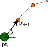
The path is the list of coordinates called path. The agent moves by setting its current position to the next element of path and looks down the path by rotating to the tangent formed between the current path point and the next.
(* agent walks towards uncovered region by following path points.  \
Breaks if an escape location is discovered.  *)
walk := (
   (* shows progress of walk *)
   walkProgress = 0;


(* Agent hops from current path point to next in list.
Rotates accoring to tangent between current path point and next *)


Do[
If[escapePoints != {}, Break[]];

pt[[1]] = path[[i, 1]](* x *);
pt[[2]] = path[[i, 2]](* y *);

\[Theta] =
ArcTan[#[[1]], #[[2]]] &[{#[[i + 1, 1]] - #[[i, 1]], #[[i + 1,
2]] - #[[i, 2]]}] &@path;

(* updtae prior location list *)
AppendTo[prior, Keys[Select[env, # == "A" &]]];

(* once position has been advanced, agent looks ahead *)
look;

(* increments walk progress *)
walkProgress += 2,

{i, 1, Length[path] - scale,(*1*)2(* step size -
increase for speed at loss of precision *)}
]
);
When walking, there is a condition where if an escape point becomes available, it will break from walk and compute a new path with the nearest escape point as its target.
(* escape points - those which are at the environment boundary *)
escapePoints :=
  Select[MemberQ[#, 1] || MemberQ[#, xLen] || MemberQ[#, yLen] &][
   sightEdges];
The procedure is the same as before. Once it has reached its destination, the agent is assumed to have escaped and the navigation component (below) of the program ends.
(* procedure agent follows to explore and eventually escape from maze \
*)
navigate := (
  (* holds env arrays for post animation *)
  sessionData = {};
  (* initilize path *)
  path = {};
  (*infoData={};*)
  (* init. status *)
  status = "Where am I?";
  (* init. escape boole *)
  escape = False;
  (* begin navigaiton by looking straight ahead *)
  look;
  (* init. prior locations *)
  prior = Keys[Select[env, # == "A" &]];


  While[escape == False,
   If[(* exit if found *)# != {},
      status = "Found escape location!";
      (* set path to esacpe *)
      (* select closest escape point *)
      verticeTarget = Nearest[#1, verticeLocation, 1][[1]];
      (* compute path *)
      computeOptimalPath;
      (* update status *)
      status =
       Row[{"Walking to escape location",
         Dynamic[{walkProgress, (Length[path] - scale)}]}];
      (* initilize walk progress *)
      walkProgress = 0;
      (* walk along path *)
      Do[
       pt[[1]] = path[[i, 1]];
       pt[[2]] = path[[i, 2]];
       \[Theta] =
        ArcTan[#[[1]], #[[2]]] &[{#[[i + 1, 1]] - #[[i, 1]], #[[i + 1,
               2]] - #[[i, 2]]}] &@path;
       look;
       walkProgress += 2,
       {i, 1, Length[path] - scale, 2}
       ];
      (* once complete,
      agent has reached destination and thus escaped *)
      escape = True;
      (* update status *)
      status = "Escaped!",

      (* if exit is not visible, then: *)
      (* explore *)

      (* perfrom complete rotation while looking *)
      status = "Looking for place to explore";
      rotateSearch;

      (* search complete,
      calculate paths from current position to valid targets *)
      status = "Deciding where to go";

      (* `pathChoices` holds target point and it's path score *)
      pathChoices = {};
      Do[
       (* valid targets are held in `opt` *)
       verticeTarget = opt[[i]];
       computeOptimalPath;
       (* calculate path score and append to list for review *)
       AppendTo[
        pathChoices, {verticeTarget,
         pathLength[path] - backtrack[path]}],
       {i, 1, Length[opt]}
       ];
      (* choose the target with maximal score and set as intended \
target *)
      verticeTarget = First[Last[SortBy[pathChoices, Last]]];

      status = "I think I'll go there";

      (* compute path to target *)
      computeOptimalPath;
      status =
       Row[{"Walking",
         Dynamic[{walkProgress, (Length[path] - scale)}]}];

      (* moves agent along path,
      breaks if exit location is discovered *)
      walk

      ] &[

    (* defines valid escape points *)
    escapePoints

    ]
   ];

  )
While agent is navigating, evaluating infoView in a subsession will give snapshots of what the agent is doing in greater detail.
Conclusion
While in need of much refinement, the program delivers good results when it works. The pathfinding algorithm has been a source of many error messages and will be the first thing to revise when I return to this project in the future. The program could be modified so that the agent searches for a key for instance before escaping or collects things in general (leading to knapsack problem). A multi-agent approach would also be interesting, especially if they could share knowledge of the maze during navigation and organize their paths efficiently. And of course, some of the methods from this project will be adapted towards traffic modelling, particularly with avoiding stopping vehicles and performing an overtake manoeuvre.
Until then, this project is being left as a functional prototype and I think Ill go back and revise my prior work with the board game Monopoly.
P.S Place notebook in a directory containing folders titled Maps and Output if using save/load features. The JSON file contains the maze shown at the start of this post.
 Attachments:


