The general question is: does NDSolve Finite Elements support coordinate systems other that Cartesian (x,y,z)?

Let's start from the very beginning with the physical model and a code to understand, how did I come to this question. First of all, I would like to note, that I'm not interested in any analytical solutions for my PDE, because the described example is only the first and trivial step of my research. Later I would like to add more terms into the PDE, like bulk chemical reaction and chemical reaction on the surface, which will make any analytical solution impossible.

So, the task is to model the diffusion-sedimentation problem for diluted dispersion of nanoparticles in liquid. The geometry I'm interested in is the standard 2 ml PP tube, like this one:

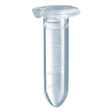
It contains of almost half-spherical part at the bottom and a cylindrical part at the top. When put vertically, this geometry has a rotational symmetry, so the obvious coordinate system for this model will be cylindrical (r, theta, z), where r is the distance from the axis of the tube and z is the height position. Because of the symmetry, theta does not matter and we could solve the problem in 2D plane (r, z).

The diffusion-sedimentation phenomenon could be described with modified Second Fick's law according to Mason,1924 (the paper is attached to this post). Indexes are omitted for clearance, later we'll define everything correctly:
D[Conc,t] - Div[Diff*Grad[Conc] - {0,0,Sv} Conc]==0, where Diff is diffusion coefficient of the particle, Sv is settling velocity of the particle, Conc is the concentration of particles at a given point in a given time. The part inside the Div is a negative flux of particles from both diffusion and sedimentation. Let's write everything correct for Mathematica. We'll use cylindrical coordinates. Also Conc is not a function of theta due to symmetry as it was described earlier:

op = \!\(
\*SubscriptBox[\(\[PartialD]\), \(t\)]\(Conc[t, r, z]\)\) - 
  Div[Diff Grad[Conc[t, r, z], {r, \[Theta], z}, "Cylindrical"] - {0, 
      0, Sv} Conc[t, r, z], {r, \[Theta], z}, "Cylindrical"]

If we evaluate this input, we get the right PDE for this case:

Sv (Conc^(0,0,1))[t,r,z]-Diff (Conc^(0,0,2))[t,r,z]-(Diff (Conc^(0,1,0))[t,r,z])/r-Diff (Conc^(0,2,0))[t,r,z]+(Conc^(1,0,0))[t,r,z]

Ok, now let's define all the constants:

T = 4; (* Temperature in deg C *)
d = 100; (* Particle's diameter in nm *)
\[Eta] = Exp[-3.7188 + 578.919/(T + 273.15 - 137.546)]; (* Vogel equation for water viscosity in mPa*s \
http://ddbonline.ddbst.de/VogelCalculation/VogelCalculationCGI.exe?component=Water *)
Diff = (1.3806485 (T + 273.15))/(3 \[Pi] \[Eta] d)*10^-7 (* Particle's diffusion coefficient in cm^2/s *)
r0 = 0.475;  (* Tube radius in cm *)
C0 = 1*10^10;  (* Initial concentration in particles/cm^3 *)
Vt = 0.5;  (* Total volume of solution *)
h = (Vt - (4 \[Pi] r0^3)/6)/(\[Pi] r0^2); (* Height of the cylindrical part in cm *)    
d\[Rho] = 0.15; (* Density difference between particle and the water in g/cm^3  *)
g = 9.807;  (* g in m/s^2 *)
Sv = -10^-10 ((g d\[Rho] (d^2) )/(18 \[Eta])) (* Settling velocity in cm/s. It's negative because z axis is pointing upwards, while settling velocity vector points  downwards *)

We'll define z=0 at the border between spherical and cylindrical parts of the tube. So z=-r0 at the bottom of the tube and z=h at the liquid surface. Although NDSolve could create a mesh automatically, I prefer to create my own mesh for this geometry. The parametric GenF function is used in order to be able to generate the mesh, which is more frequent close to tube wall, which is required for further more complex models with reactions on the surface with sharp gradients near the wall.

<< NDSolve`FEM`
NCyR = 100;
NCyZ = 10;
NSphR = 10;
GenF=r0 (1-Exp[-9#])&;
(* Coords definition for cylindrical part *)
CyCoord = Flatten[Append[Table[{GenF[x], z}, {x, 0, 1, 1/(NCyR - 2)}, {z, 0, h,h/(NCyZ - 1)}], Table[{r0, z}, {z, 0, h, h/(NCyZ - 1)}]],1];
(* Inc definition for cylindrical part *)
CyInc = Flatten[Table[{j*NCyZ + i, j*NCyZ + i + 1, (j - 1)*NCyZ + i + 1, (j - 1)*NCyZ + i}, {i, 1, NCyZ - 1}, {j, 1, NCyR - 1}], 1];
(* Coords for spherical part *)
SphCoord = Flatten[Append[Table[{-GenF[x] Sin[\[Phi]], -GenF[x] Cos[\[Phi]]}, {x, 1/(NCyR - 2), 1, 1/(NCyR - 2)}, {\[Phi], 0, -\[Pi]/2, -\[Pi]/2/(NSphR - 1)}], Table[{-r0 Sin[\[Phi]], -r0 Cos[\[Phi]]}, {\[Phi], 0, -\[Pi]/2, -\[Pi]/2/(NSphR - 1)}]], 1];    
SphCoord = Prepend[SphCoord, {0,0}]; 
(* Calculate the shift of the spherical coordinates *)
SphSh = Length[CyCoord];
(* Inc definitions for spherical part *)
SphInc = Flatten[Table[{j*NSphR + i + 1, j*NSphR + i + 2, (j - 1)*NSphR + i + 2, (j - 1)*NSphR + i + 1}, {i, 1, NSphR - 1}, {j, 1, NCyR - 2}], 1]; 
SphTrInc = Table[{i + 1, i + 2, 1}, {i, 1, NSphR - 1}];

FullMesh = ToElementMesh["Coordinates" -> Join[CyCoord, SphCoord], "MeshElements" -> {QuadElement[CyInc], 
     TriangleElement[SphTrInc + SphSh], QuadElement[SphInc + SphSh]}];
FullMesh["Wireframe"]

This code generates the 2D-mesh like the one attached to this post. Looks good. Now let's define initial conditions (homogeneous solution with Conc = C0) and solve the PDE with NDSolve. We should also define boundary conditions of zero particles flux as a NeumannValue, but NDSolve should do it automatically. We'll also plot this solution after 48 h.

ic = Conc[0, r, z] == C0;
sol = NDSolve[{op == 0, ic}, Conc, {t, 0, 48*3600}, {r, z} \[Element] FullMesh][[1]]

TSection = 48; (* Visualization time in hours *)
VisRZCoord = FullMesh["Coordinates"];
VisTable = Table[{VisRZCoord[[i, 1]], VisRZCoord[[i, 2]], With[{t = 3600 TSection, r = VisRZCoord[[i, 1]], z = VisRZCoord[[i, 2]]}, Evaluate[Conc[t, r, z] /. sol]]}, {i, Length[VisRZCoord]}];
ListPlot3D[VisTable, PlotRange -> {All, All, {0, 1.1 C0}}, PlotLabel -> "t = " <> ToString[TSection] <> " h"]

The resulted 3D plot is attached to the post as "48 h, 100 nm.png". It looks flat and that's strange, because there must be a gradient of concentration due to sedimentation. Let's change the diameter of the particles to 1000 nm (1 mkm) and density difference to 1 g/cm^3. This definitely should cause the sedimentation. NDSolve generates the warning of large Peclet number (this is Ok, we could handle this if it will be necessary), but the 3D plot stays the same.

It looks like NDSolve wrongly set up the NeumannValue for my PDE. It nullifies the diffusion flux only, so the 3D-plot makes sense: there is a constant sedimentation flux of particles over the upper boundary and the lower boundary. That's why the concentration stays constant. Well, that's a good result, but this isn't the model I'm interested in. The solution for this problem, that could be found in many places, is to inactivate the Div, Grad and Plus during the PDE definition. Let's revert particle diameter and density difference back (to 100 nm and 0.15 g/cm^3) and try Inactivate:

op = \!\(\*SubscriptBox[\(\[PartialD]\), \(t\)]\(Conc[t, r, z]\)\) - Inactive[Div][Inactive[Plus][Inactive[Times][Diff, Inactive[Grad][Conc[t, r, z], {r, \[Theta], z}, "Cylindrical"]], Inactive[Times][{0, 0, -Sv}, Conc[t, r, z]]], {r, \[Theta], z}, "Cylindrical"]
ic = Conc[0, r, z] == C0;

Now NDSolve says:

Inactive::argrx: Inactive[Div] called with 3 arguments; 2 arguments are expected. >>

A strange error. I can't find it in help or tutorials. I can't find it with Google as well. By definition, Div could be called with 3 arguments. I've looked through all the available examples in help and tutorials and found, that there isn't any examples with coordinates other than Cartesian. So I proposed, that coordinate systems other than Cartesian are simply not implemented for Finite Elements in Mathematica 10.2.0 yet and this error is just a dummy. That's how I came to my original question.

Any ideas how to make this work?

P.S. I also tried to include the theta as the variable for Conc explicitly. Something like this:

op = \!\(\*SubscriptBox[\(\[PartialD]\), \(t\)]\(Conc[t, r, 0, z]\)\) - Inactive[Div][Inactive[Plus][Inactive[Times][Diff, Inactive[Grad][Conc[t, r, 0, z], {r, \[Theta], z}, "Cylindrical"]], Inactive[Times][{0, 0, -Sv}, Conc[t, r, 0, z]]], {r, \[Theta], z}, "Cylindrical"]
ic = Conc[0, r, 0, z] == C0; 

But this wasn't an issue, I've got the same Inactive::argrx: error.

Attachments: