Abstract
The goal of this project is to implement the Huffman lossless data compression algorithm which is a compression algorithm based on the frequency of data. The trick is that the words which are more commonly used must be shorter than the words which are less common. The English language already uses this approach, for example, the word "the" is frequently used and short but the word "approximation", which is much less frequent is longer.
- Introduction to Huffman coding
- Word frequency data
- Huffman algorithm code in Mathematica and a few examples
- Correlation between words and Huffman codes
Introduction to Huffman coding
Huffman coding is a statistical technique, which attempts to reduce the amount of bits required to represent a string or a symbol. The concept of Huffman algorithm is that the shorter binary codes are assigned to the most frequently used symbols and longer codes to the symbols which appear less frequently. The Huffman code for an alphabet (set of symbols or words) may be generated by constructing a binary tree with nodes containing the symbols to be encoded and their probabilities of occurrence (that's where the statistical part comes in). This means that you must know all of the symbols that will be encoded and their probabilities prior to constructing a tree. In computer science and information theory, a Huffman code is a particular type of optimal prefix code that is commonly used for lossless data compression. The algorithm was originally developed by David A. Huffman.
Word frequency data:
As an input for the Huffman coding algorithm, we use the 5000 most frequently used words in English. See the database Here. The following is the visualization of most commonly used words,
$\qquad \qquad \qquad \qquad \qquad \qquad $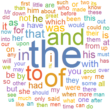
Examples of Huffman codes
merge[k_] :=
  Replace[k, {{a_, aC_}, {b_, bC_}, rest___} :> {{{a, b}, aC + bC},
     rest}];

mergeSort[d_List] := FixedPoint[merge @ SortBy[#, Last] &, d][[1, 1]];

findPosition[l_List, k_List] := Map[
    (# -> Flatten[Position[k, #] - 1]) &,
    DeleteDuplicates[l]
];

huffman[l_List] := Module[{sortList, code, words},
  words = l[[All, 1]];
  sortList = mergeSort[l];
  code = findPosition[words, sortList];
  {Flatten[l /. code], code};
  code
]
These are a few examples of encoded words using Huffman algorithm
$\qquad \qquad \qquad \qquad \qquad \qquad $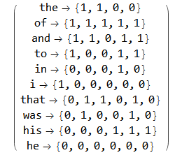
Correlation between words and Huffman codes
The following is the correlation plot of the numbers of letters in a word and number of bits produced by Huffman algorithm. As you can see from the plot the most commonly used words in English tend to be shorter and the overall the trend in English and in Huffman code is the same.
$\qquad \qquad \qquad \qquad \qquad \qquad $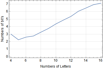
The following plot represents the number of bits of English words and the number of bits of Huffman codes. The number of bits per English word was computed using a conversion factor of $\log_2(26) ~ 4.7$ bits per word, where 26 is the number of letters in the English alphabet.
$\qquad \qquad \qquad \qquad \qquad \qquad $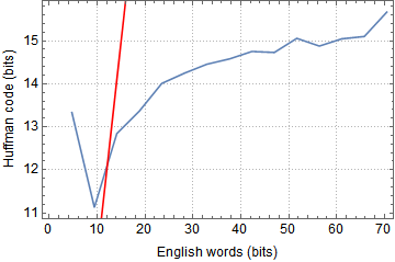
The blue line is a scatter plot of the number of bits in English versus the number of bits in the Huffman code. The red line is $y=x$. .As you can see the Huffman coding is much more efficient and the slope of the curve tells us that the Huffman coding uses three times less space than the English language.
 Attachments:


