Abstract

La Liga is underway. Millions of fans are looking forward to their favorite teams and players. As every year, 20 clubs will struggle to win one of the most prestigious titles in Europe, and with the start of the league, many gamblers will also try to prove themselves worthy by betting on the matches. This project aims at developing a program which can give betting predictions on the upcoming matches of the league. It is implemented using machine learning techniques and the broad tool-set that is provided by Mathematica. The full source code of this project can be downloaded from here. To accomplish our goal we collected data to feed the algorithms of the machine learning functions Predict and Classify. We crawled data of the last 6 seasons (all matches in between 2010 and 2016) of Spanish League from a sports statistics website using Scrapy [1]. The data includes more than 2200 matches along with numerous relevant statistics. After that the data passed through multiple stages of refinement. Since for a single match there are numerous odds on different events (e.g. total goals, outcome, odds for goalscorers etc) we decided to keep it simple and chose to predict the outcome - one the most common events. We computed and added to the data several specific features, such as ratings, head to head statistics, that mostly affect the rightness of corresponding event. After adjusting the data we used built in Mathematica functions Predict and Classify to predict the events. These functions are used to give suggestions on the outcome of the match. We then tested our predictions on the actual odds of our matches. The odds were crawled from another website which contained all of the winning odds of Spanish League matches played in between 2010 to 2016. This data allowed us to simulate betting and try to estimate the profitability of our program. Finally, based on our calculations we suggest betting strategies that satisfy the most optimal risk-profit relationship.

Data Transformation And Filtering

Data Transformation

To start with, we imported our csv formatted match data and the ratings into Mathematica. Below is shown a sample of the match data csv file.

match_date,team_1,team_2,team_win,coef_1,coef_x,coef_2,coef_win,score 15-05-2016,Betis,Getafe,Betis,3.49,3.73,2.06,3.49,2:1 15-05-2016,Gijon,Villarreal,Gijon,1.50,4.64,6.31,1.50,2:0 15-05-2016,Rayo Vallecano,Levante,Rayo Vallecano,1.36,5.77,7.60,1.36,3:1 15-05-2016,Espanyol,Eibar,Espanyol,2.05,3.68,3.75,2.05,4:2 15-05-2016,Malaga,Las Palmas,Malaga,1.69,3.94,5.17,1.69,4:1

Then we used the function SemanticImport, which returns a Mathematica dataset. From the match data we imported 8 columns which are team_1, team_2, date, score etc. Then we did data cleaning to make it easier to work later.

oddsData = SemanticImport[
         "/home/mher/Desktop/BPS_Project/Data/oddsportal_selenium/output.csv",
         <|1->"Date",2->"String",3->"String",5->"String",6->"String",7->"String",8->"String",9->"String"|>
       ];

oddsToNumbers[a_Association]:=
    If[
    StringCount[a["coef_1"],"/"]== 0,
    ReplacePart[a,
       {
         "coef_1" ->ToExpression[a["coef_1"]],
         "coef_x" ->ToExpression[a["coef_x"]],
         "coef_2" ->ToExpression[a["coef_2"]],
         "coef_win" ->ToExpression[a["coef_win"]]
       }
    ],
    ReplacePart[a,
       {
         "coef_1" ->N[Divide @@ Map[FromDigits,StringSplit[a["coef_1"],"/"]] ,2] + 1.,
         "coef_x" ->N[Divide @@ Map[FromDigits,StringSplit[a["coef_x"],"/"]] ,2] +  1.,
         "coef_2" ->N[Divide @@ Map[FromDigits,StringSplit[a["coef_2"],"/"]] ,2] +  1.,
         "coef_win" ->N[Divide @@ Map[FromDigits,StringSplit[a["coef_win"],"/"]] ,2] +  1.
       }
    ]
]

oddsData=Map[oddsToNumbers,oddsData];
oddsData=Dataset[KeyMap[StringJoin[Capitalize[StringSplit[#,"_"]]]&,#]& /@ Normal[oddsData]];

With a simple function we extract the individual goals scored from both teams.

extractGoals[a_] :=
    Append[a,
     <|
         "Team1Goals" -> FromDigits[StringSplit[a["Score"], ":"][[1]]],
         "Team2Goals" -> FromDigits[StringSplit[a["Score"], ":"][[2]]]
        |>
    ]

oddsDataNew = Map[extractGoals[#] &, oddsData];

Now data is ready. The code below adds a new column named GoalsTotal to our dataset to provide the total goals for every match. Afterwards with the function addRating we add the ratings for each club in the league.

dataNew = oddsDataNew[All,

   Append[#,
     "GoalsTotal" -> Slot["Team1Goals"] + Slot["Team2Goals"]] &];

ratingsRawForOddsData = SemanticImport[
    "/home/mher/Desktop/BPS_Project/Data/oddsportal_selenium/ratings_for_odds_data_names.csv",
    <|1 -> "String", 2 -> Automatic|>];

ratings = AssociationThread @@ Transpose[Values /@ Normal[ratingsRawForOddsData]];

addRating[d_] :=
  Join[d,
   Association[
    "Team1Rating" -> (ratings[d["Team1"]]),
    "Team2Rating" -> (ratings[d["Team2"]])
    ]
   ];

ratingsAdded = Map[addRating[#] &, dataNew] ;

Now that we have added the ratings and total goals we can start to compute some individual features for every team and add them to our dataset. To accomplish that we first group all the matches by home and away status for every team. Afterwards we add to our dataset a very important data column - the individual total goals average per match. This feature is essential for predicting the total goals of a certain match (the prediction of total goals is not included in this post, it will be published later).

homeAndAway =
  dataNew[
   Association[
    "Home" -> GroupBy[#Team1 &],
    "Away" -> GroupBy[#Team2 &]
    ]
 ];

addIndividualTotalGoalsAvrgs[d_] :=   
  Join[d,
    Association[
    "Team1TotalAvrg" ->
    (N[Mean[Join[homeAndAway["Home", d["Team1"], All, "Team1Goals"],
         homeAndAway["Away", d["Team1"], All, "Team2Goals"] ]], 3]),
    "Team2TotalAvrg" ->
    (N[Mean[Join[homeAndAway["Away", d["Team2"], All, "Team2Goals"],
         homeAndAway["Home", d["Team2"], All, "Team1Goals"]]], 3])
    ]    
];

avrgsAdded = Map[addIndividualTotalGoalsAvrgs[#] &, ratingsAdded];

Another powerful parameter for predicting the total goals is the total number of goals that were scored during head to head clashes of two specific teams.

 addHeadToHeadTotalGoalsAvrg[a_] :=
 Append[a,
  "H2HTotalAvrg" ->
    (N[Mean[Select[avrgsAdded,
        Or[And[#Team1 == a["Team1"] , #Team2 == a["Team2"]] ,
          And[#Team1 == a["Team2"], #Team2 == a["Team1"]]] &][All, "GoalsTotal"]], 3])
 ]

headToHeadTotalGoalsAvrg = Map[addHeadToHeadTotalGoalsAvrg[#] &, avrgsAdded];

One of the most influential factors that affect the outcome of a match is the home and away statuses of the teams. The reason behind is that relatively weak teams tend to play better at home stadium.

addHomeTeamStatus[a_] :=
    Append[a,
         "HomeTeam" -> "Team1"
  ]

homeStatusAdded = Map[addHomeTeamStatus[#] &, headToHeadTotalGoalsAvrg];

Continuing the data transformation we added the outcomes of the matches. We give them numerical values: 1 for the win of the home team, -1 for the win of the away team and 0 for draw. This choice makes no difference in case of the classification done by the function Classify. However, it is crucial for predicting the outcome with the function Predict. Obviously, when needed, we can always remap the numerical values to the three outcome categories. Another important advantage of using numeric outcomes is that it allows to add Head to Head statistics feature which numerically shows which team has advantage over its opponent in previous matches. Eventually we are going to compare the accuracies when using categorical and numerical outcomes.

addOutcome[a_Association] :=
 If[
      a["Team1Goals"] == a["Team2Goals"],
      Append[a, Association["Outcome" -> 0]],
      If[a["Team1Goals"] > a["Team2Goals"],
           Append[a, Association["Outcome" -> 1]],
           Append[a, Association["Outcome" -> -1]]
   ]
  ]

outcomeAdded = Map[addOutcome[#] &, homeStatusAdded];

Data Filtering

In this phase of the data processing we add one more valuable feature which is Head to Head statistics. It basically illustrates the advantage of Team1 over Team2 during their previous matches. Then we filter the data based on the minimum number of total matches played between two specific teams.

possibleMatches = DeleteDuplicates[Values@Normal@outcomeAdded[All, {"Team1", "Team2"}]];

headToHeadTotal[t1_, t2_] :=
 Mean[
  Join[
   Normal@
    outcomeAdded[Select[#Team1 == t1 && #Team2 == t2 &],"Outcome"],
    - Normal[outcomeAdded[Select[#Team2 == t1 && #Team1 == t2 &], "Outcome"]]
   ]
  ]

h2hAdded = outcomeAdded[All, Append[#, "H2H" -> (headToHeadTotal[#Team1, #Team2])] &];

filterLowStatistics[t_?NumberQ] := filterLowStatistics[#, t] &
filterLowStatistics[list_, t_] :=
 Module[
  {matches, counts, toKeep},
  matches = Sort /@ Lookup[list, {"Team1", "Team2"}];
  counts = Replace[matches, Counts[matches], {1}];
  toKeep = Thread[counts > t];
  Pick[list, toKeep]
  ]

filteredData = h2hAdded[filterLowStatistics[1]];

Here are the first ten rows and all the added columns of our dataset.

Building the Classifier of Outcome

Now we can initialize and train our classifier. There are 3 categories for the outcome of the match, namely 1 for Team1 victory, -1 for Team2 victory and 0 for the Draw. Here the dataset is separated into the training set and the test set. The columns which represent features that are relevant in predicting the outcome are HomeStatus, Team1Rating, Team2Rating and head to head statistics, labeled as H2H.

n = Round[0.9Length[filteredData]];
{trainingSet,testSet}=TakeDrop[filteredData[All,{"HomeTeam","Team1Rating","Team2Rating","H2H","Outcome"}],n];

c = Classify[trainingSet->"Outcome",Method->"LogisticRegression"]

Here we use the function ClassifierMeasurements to check the accuracy of our classifier.

cm = ClassifierMeasurements[c, testSet -> "Outcome"]

cm["Accuracy"]
0.657895

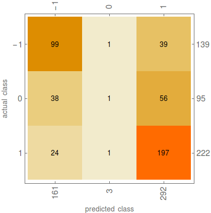
The classification accuracy is almost 66%. This number shows how powerful is the head to head statistics feature. Without this feature the accuracy would only be 58%. Now let's look at the confusion matrix plot which is very useful feature of ClassifierMeasurements function and allows to analyze the wrong classifications of the created model.

cm["ConfusionMatrixPlot"];

From the plot we can see that our classifier does not tend to predict Draw as an outcome.

Let's analyze the results a bit. By subtracting the outcomes of actual and predicted numerical classes we get a list named difference which contains integers from -2 to 2. If the subtraction of actual and predicted values is 0 then the classification was valid. Numbers -2, -1, 1 and 2 are the matches which were classified incorrectly.

actaulValue=testSet[All,"Outcome"] //Normal;
predictedValue=c[testSet];
difference=actaulValue - predictedValue;

N @ Normalize[Counts[Abs[difference]],Total]
<|0 -> 0.657895, 1 -> 0.192982, 2 -> 0.149123|>

Continuing with the analysis we see that more than 65% of the matches in the testSet were classified correctly. The rest of the matches were classified incorrectly but with a little difference. The matches that have value 1 in the difference list were classified wrongly with just 1 step of miss. Let us bring an example to make this a bit clearer. Let's take a match to which corresponds a value of 1 in the difference list. If our classifier predicted victory of Team1 and it missed (obviously) that means the match was drawn, because the difference of actual and predicted values is 1. Similarly, we can state that nearly 15% of the matches were totally misclassified, because the absolute value of the difference is 2.

Building the Predictor of Outcome

At this part of the project we use a different approach to find out the outcome of the match. Now we don’t try to predict the category of outcome as in case of the function Classify, but rather a numerical outcome on an axis that goes from -1 (win), to 1 (loss), where values close to 0 are interpreted as draws. Similar to the method used in previous section we prepare the training and test sets.

n = Round[0.8 Length[filteredData]]
1822

{trainingSetFull, testSetFull} = TakeDrop[filteredData, n];
{trainingSet, testSet} = {trainingSetFull[All, {"Team1Rating", "Team2Rating", "H2H", "Outcome"}], testSetFull[All, {"Team1Rating", "Team2Rating", "H2H", "Outcome"}]};

We train the function and then we use the function PredictorMeasurements to test our prediction on some test data.

p = Predict[trainingSet -> "Outcome"]

pm = PredictorMeasurements[p, testSet -> "Outcome"]

Now let' s run the predictor on our test to see what it does predict.

Max[p[testSet]]
Min[p[testSet]]

1.26189
-0.872063

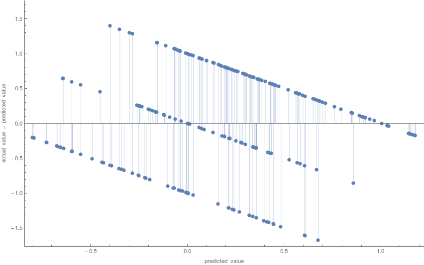
So we got numerical values for the outcomes of the matches. It gave values ranging from roughly - 0.8 to 1.2. Later on we will write a function to convert the numerical values to categories but for now let us analyze the ResidualPlot of our predictor.

pm["ResidualPlot"]

The plot above shows the difference between actual and predicted values for the outcome of the matches of the test set. Every point represents a single game. We can state that points that lie on y=0 which represent difference equal to 0 are the perfect guesses. Moreover points that lie near the 0 axis are almost perfect guesses. All other points have a certain amount of distance from 0 which basically shows how far the predictions were from the right guess. Continuing with the outcome predictor, we must convert the numerical values of the predictor into 3 categories based on the results of the residual plot. For now we only will create a very rough approximation to see how much accuracy we can get.

actual = testSet[All, "Outcome"] // Normal;
outcomeBackToClasses = Function[UnitStep[# - .2] - UnitStep[-# - .2]];

Here we classified the predicted numbers in range (-0.2 ; 0.2) as 0-s. Moreover numbers greater than 0.2 are now classified as 1s and those less than -0.2 to -1-s. Similar to the method we used in case of the Classifier, we try to find out the accuracy of prediction as well as how bad our predictor did in the cases of wrong predictions.

predictedOutcome = outcomeBackToClasses[p[testSet]] ;

dif = actual - predictedOutcome;

N @ Normalize[Counts[Abs[dif]], Total]

<|0 -> 0.631579, 2 -> 0.0964912, 1 -> 0.27193|>  

Although the accuracy of our classifier has decreased slightly we see a fundamental improvement in totally missed guesses which are represented with number 2. The percentage of total misses decreased from 15% to 0.09%. Another advantage that the predictor has over the classifier is that now it also guesses reasonable amount of draws. Those advantages are very effective in betting, because draws are considered difficult events to predict and usually odds for draws are much higher than those for wins.

Betting Simulation and Strategies

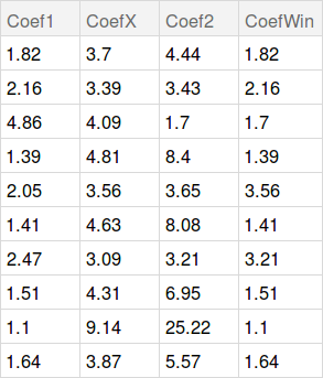
Here we start probably the most interesting part of the project—betting simulations. As it was mentioned above, our data has all the odds for the outcomes of all the matches of the league. There are 4 columns for the odds— win of Team1, win of Team2, Draw and the wining coefficient - CoefWin. Here is a sample of the odds data.

Now let's simulate simple bets. To do that we randomly choose 10 matches and give them to our predictor to guess the outcome. As a result we get numerical values which we then convert into three classes with the help of the piece-wise function. After that we get a list containing 1s, -1s and 0s. Those are the outcomes that the predictor guessed for randomly selected 10 matches.

randomMatches = RandomSample[testSetFull, 10];

p[randomMatches[All, {"Team1Rating", "Team2Rating", "H2H", "Outcome"}]]
{0.459584, -0.0321182, 0.967641, 0.459716, 1.04778, 0.201723, 0.399631, -0.0359151, 0.831428, -0.085207}

randomMatchesPredicted = outcomeBackToClasses[p[randomMatches[All, {"Team1Rating", "Team2Rating", "H2H", "Outcome"}]]]
{1, 0, 1, 1, 1, 1, 1, 0, 1, 0}

Than we write a rule and convert the guesses to the corresponding coefficients.

randomMatchesPredicted /. {0 -> "CoefX", 1 -> "Coef1", -1 -> "Coef2"}
{"Coef1", "CoefX", "Coef1", "Coef1", "Coef1", "Coef1", "Coef1", "CoefX", "Coef1", "CoefX"}

Let's remember how we determined the correct guesses. We simply checked if the difference between predicted and actual class is 0 or not. Therefore we construct a function that takes the difference between actual and predicted classes as an argument and returns 1 if and only if the difference is 0. Than we multiply the result of that function to the corresponding winning odds. This way we simulate a bet of 1 dollar for every match. That function is

1 - Abs[Sign[dif]]

Here is the result of the multiplication

(1 - Abs[Sign[Normal@randomMatches[All, "Outcome"] - randomMatchesPredicted]]) Normal @ randomMatches[All, "CoefWin"]
{1.93, 3.26, 1.15, 2.38, 1.11, 1.37, 1.36, 3.12, 1.88, 0.}

So the question is weather we actually win? To figure that out we do Total of the won money and then subtract from it the 10 dollars we have bet in total (1 dollar for a match).

Total[%] - 10
7.56

Booom. We won 7.56 dollars. However, do not rush to gamble. This process is purely probabilistic. That is, we could also lose money firstly because we have 66% of accuracy. And secondly, even if we had 100% accuracy based of the data of previous matches, we could not always win on future matches. To gain a better understanding of how profitable this kind of betting is, one needs to perform a sufficient number of betting simulations. Then only after analyzing the results and after calculating mean profit it would be possible to speak about long term wins. However, the significance in the numeric approach to the prediction of the outcome is that we can decide on what event to bet based on numeric predictions. Let me bring an example. Below are the predicted numeric values for randomly selected 10 matches.

{0.459584, -0.0321182, 0.967641, 0.459716, 1.04778, 0.201723, 0.399631, -0.0359151, 0.831428, -0.085207}

As we can see there are numbers which are near-perfect meaning those are very close to either 1, -1 or 0. For example take the 2nd and 8th numbers of the numeric predictions. Both of them are equal to -0.03, which means those are near perfect Draw guesses. So we can use this fact to make an xpressbet, which is a particular type of bet in which the player predicts multiple events and wins only if all the predicted events happen. In that case we get the odds multiplied to each other. In this particular case we try to predict 2 events. The odds for draws were 3.26 for the 2nd match and 3.12 for the 8th match so the total odd would be 10.17. And if we bet on this odd 1 dollar we earn 9 dollars, just by betting on 2 matches with an xpressbet. This strategy minimizes the risk of losing money at the same time maximizes the profit. However the probability to win falls because we have done an xpressbet. That is, we need both of the predictions to be correct. And this is where the predictor helps us to decide what are the near-perfect guesses to link and bet on. We see that the flexibility of our model allowed us to come up with some betting strategies based on the result of our numerical predictor. Definitely will be tested this weekend.

Conclusion and Future Work

• 66% accuracy for classifier
• 63% accuracy for predictor
• optimal risk-profit betting strategy
• development of total goals predictor

References

1. “Scrapy | A Fast and Powerful Scraping and Web Crawling Framework.” Accessed August 16, 2016. http://scrapy.org/.
2. Bernard, Etienne. “Posts by Etienne Bernard—Wolfram Blog.” Accessed August 18, 2016. http://blog.wolfram.com/author/etienne-bernard/.

Attachments: