Some time ago I saw a beautiful BBC documentary presented by an outstanding presenter, Hannah Fry, on "The Joy of Data". She discussed a fascinating observation: If you start at a random wikipedia page, click on the first link in the main body of the article and then iterate, you will (with a probability of over 95%) end up at the Wikipedia article on Philosophy. There is a wiki article that explains the phenomenon; it also contains a link to an online tool to check this observation for a small number of starting pages. I think that one of the best descriptions of this phenomenon are in this short clip from Hannah Fry's program.
Now, in this post I will show how to write a very crude crawler to generate networks like this:
In a certain sense this post is in a similar spirit to a post by @Sander Huisman on Roads to Lyon and another one by @Bernat Espigulé Pons on the Roads to Rome. There is this article on Letter Frequencies in Wikipedia by @Vitaliy Kaurov that animated me to write this post up now. Wikipedia is very special. It is fluid, keeps changing all the time and is a community effort that grows.
First, primitive crawler
The first thing we need to do is find the first link in each article. The Wolfram Language has Wikipedia data right built in, but I did not quite see a way of extracting the first link of the main body of the article. In
WikipediaData["Scotland", "LinksRules"]
the links are ordered alphabetically and therefore do not solve your problem.
A first example
Using a lit of (quite ugly) parsing and the powerful NestList we can get a sequence of links:
NestList[(Select[Table[Quiet[("https://en.wikipedia.org/wiki" <> StringSplit[StringSplit[StringSplit[#, "<p>"][[k]], "<a href=\"/wiki"][[2]], "\""][[1]])], {k, 2, 10}],
StringQ[#] &][[1]] &@ Import[#, "Source"]) &, "https://en.wikipedia.org/wiki/Germany", 30]
Here we start at the article for Germany and "walk" for 30 steps. Here's the result:
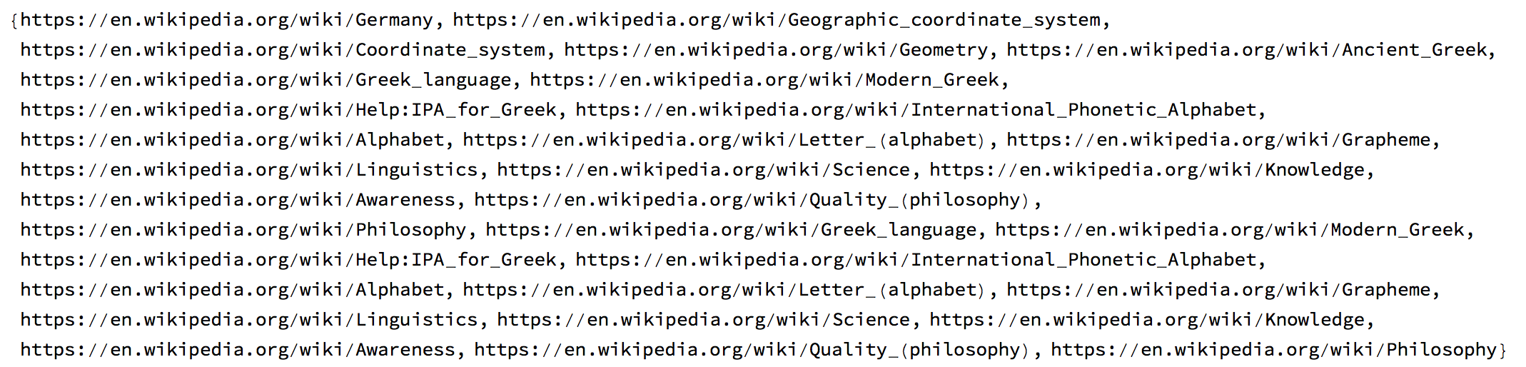
You actually see that we reach the article on Philosophy then move away and come back to it. So we end up at a sort of loop. Another problem is that we do not know for how long we have to walk before getting there (or not getting there?). We should rather use this function
startGermany =
 NestWhileList[(Select[Table[Quiet[("https://en.wikipedia.org/wiki" <> StringSplit[StringSplit[StringSplit[#, "<p>"][[k]], "<a href=\"/wiki"][[2]], "\""][[1]])], {k, 2, 10}], StringQ[#] &][[1]] &@Import[#, "Source"]) &, "https://en.wikipedia.org/wiki/Germany", UnsameQ, All]
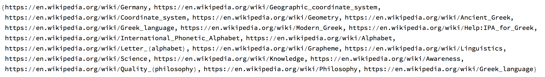
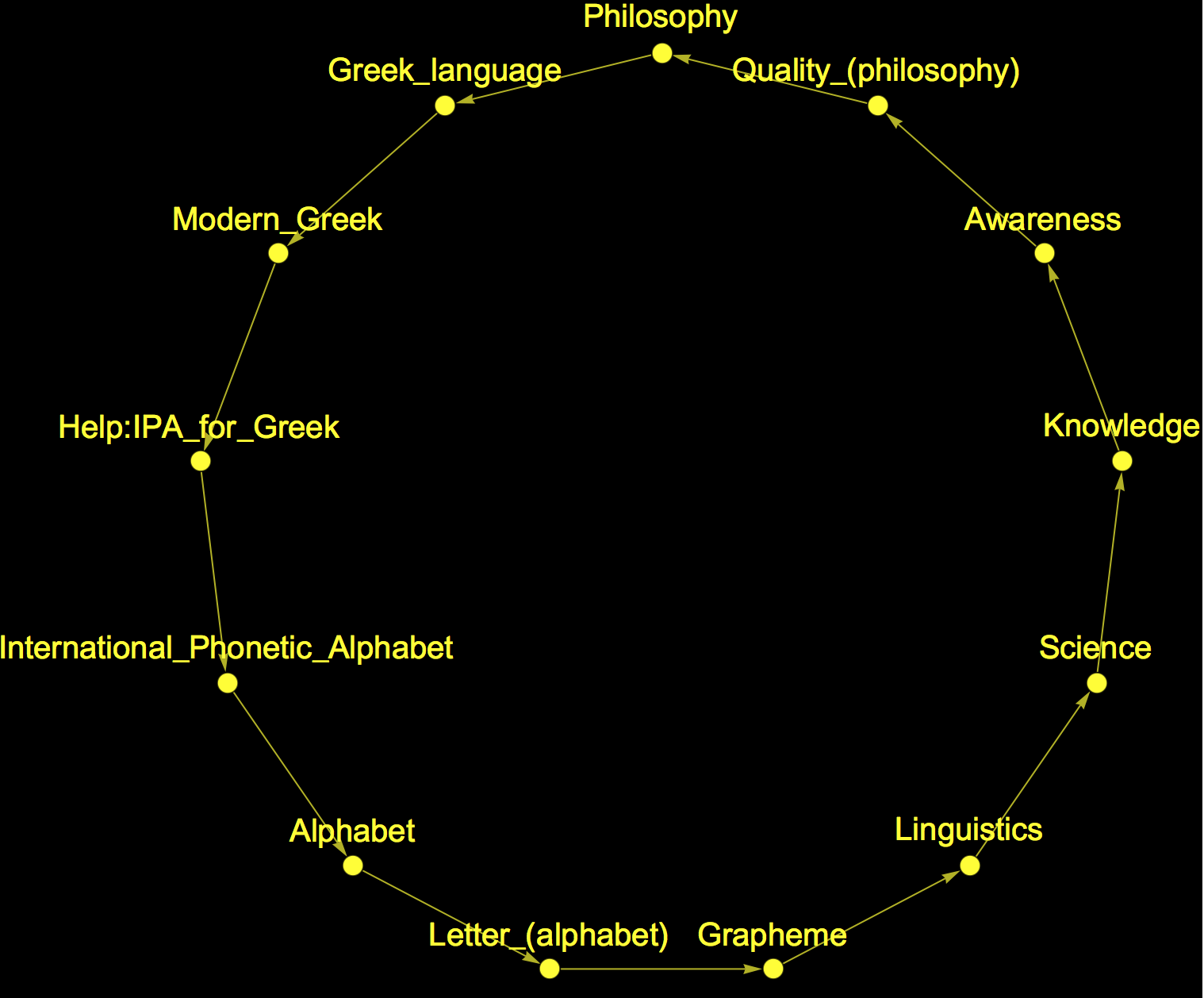
We can plot this now:
Graph[Rule @@@ Partition[StringDelete[startGermany, "https://en.wikipedia.org/wiki/"], 2, 1], VertexLabels -> "Name", ImageSize -> Full]
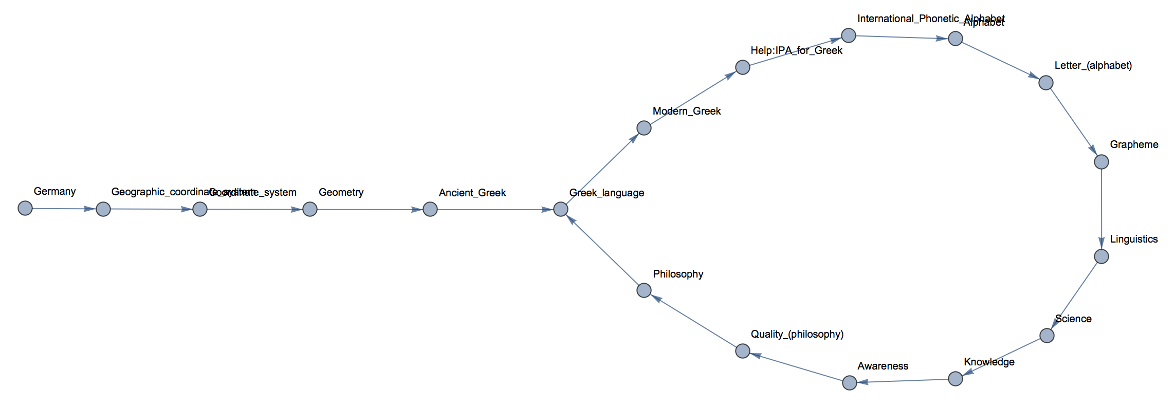
We can clearly see how we move from the first article onto a loop. The loop is a sort of attractor of the system. In fact, what we really want to study is the "basin of attraction" of this attractor, i.e. which initial pages end up on this attractor.
More systematic crawling approach
The next thing is to find suitable starting pages. Here is an implementation which uses the "random page" function built into wikipedia:
startingpages =
  Table[RandomChoice[Select[Import["https://en.wikipedia.org/wiki/Special:Random", "Hyperlinks"], (StringContainsQ[#,
  "https://en.wikipedia.org/wiki/"] && ! StringContainsQ[StringDelete[#, "https://en.wikipedia.org/wiki/"], ":"]) &]], {100}];
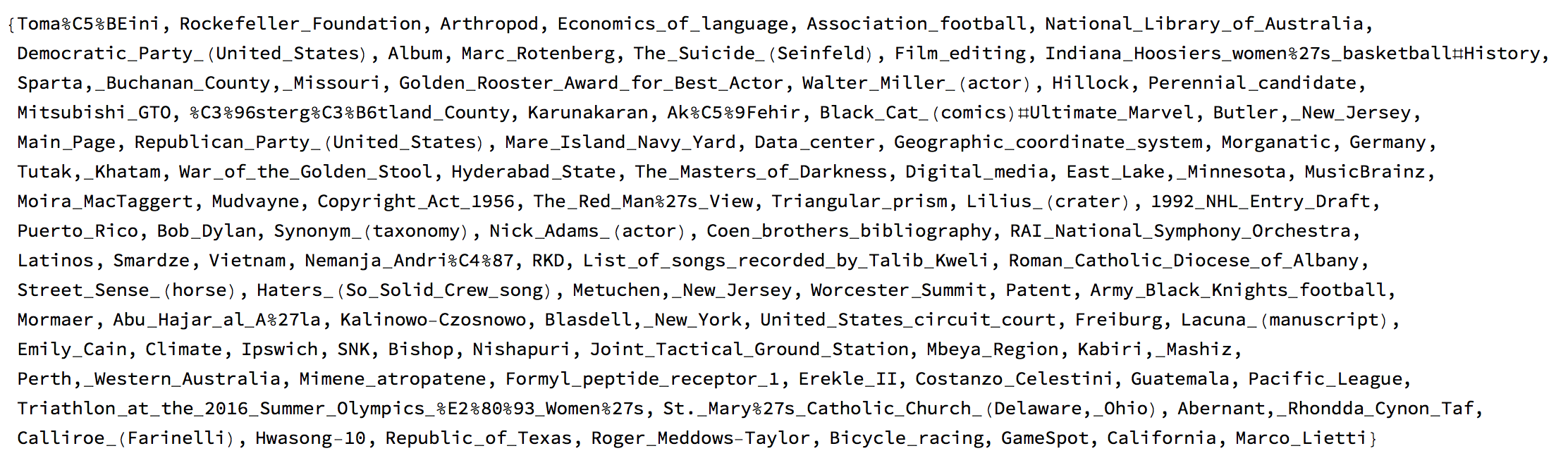
These are the articles that were randomly chosen when I ran the code:
DeleteDuplicates[StringDelete[startingpages, "https://en.wikipedia.org/wiki/"]]
Now we need to get the data. The paths of the 100 pages are relatively quick to generate:
Monitor[paths =
   Table[NestWhileList[(Select[Table[Quiet[("https://en.wikipedia.org/wiki" <>
   StringSplit[StringSplit[StringSplit[#, "<p>"][[k]], "<a href=\"/wiki"][[2]], "\""][[1]])], {k, 2, 10}],
   StringQ[#] &][[1]] &@Import[#, "Source"]) &, startingpages[[m]], UnsameQ, All], {m, 1,
   Length[startingpages]}];, m]
Note, that when you run the code you should add a Pause[...] so that you do not put the Wikipedia server under pressure. Just to be safe, I would rather also export the data, after the download:
Export["~/Desktop/startingpagessmall.mx", startingpages];
Export["~/Desktop/paths.mx", paths];
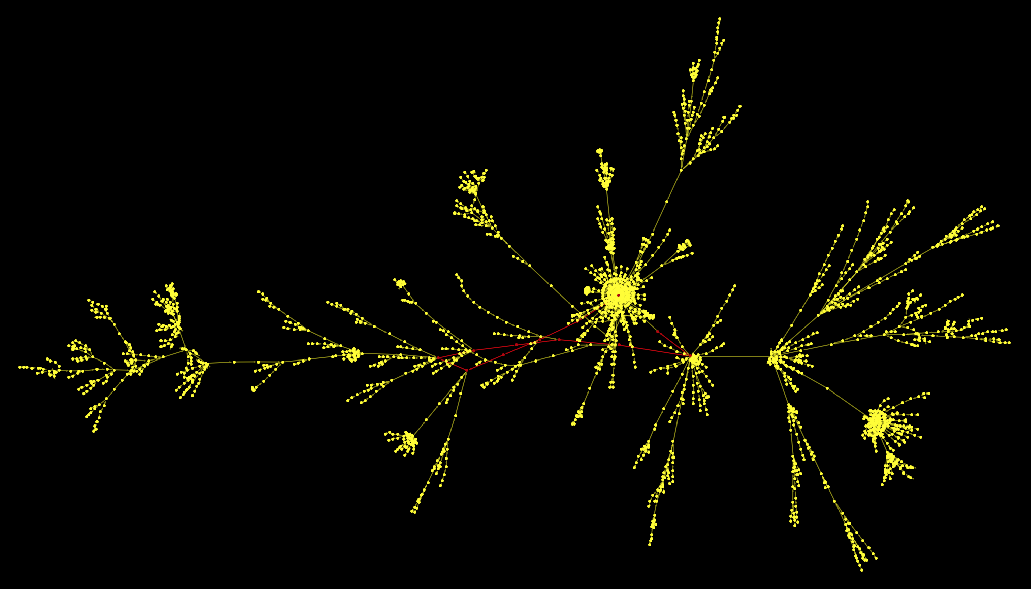
We can now plot the result of our first analysis.
HighlightGraph[
 Graph[DeleteDuplicates[
 Flatten[Rule @@@ Partition[StringDelete[#, "https://en.wikipedia.org/wiki/"], 2,1] & /@ paths]], Background -> Black, VertexStyle -> Yellow,
  EdgeStyle -> LightYellow, VertexSize -> 2, ImageSize -> Full], "Philosophy"]
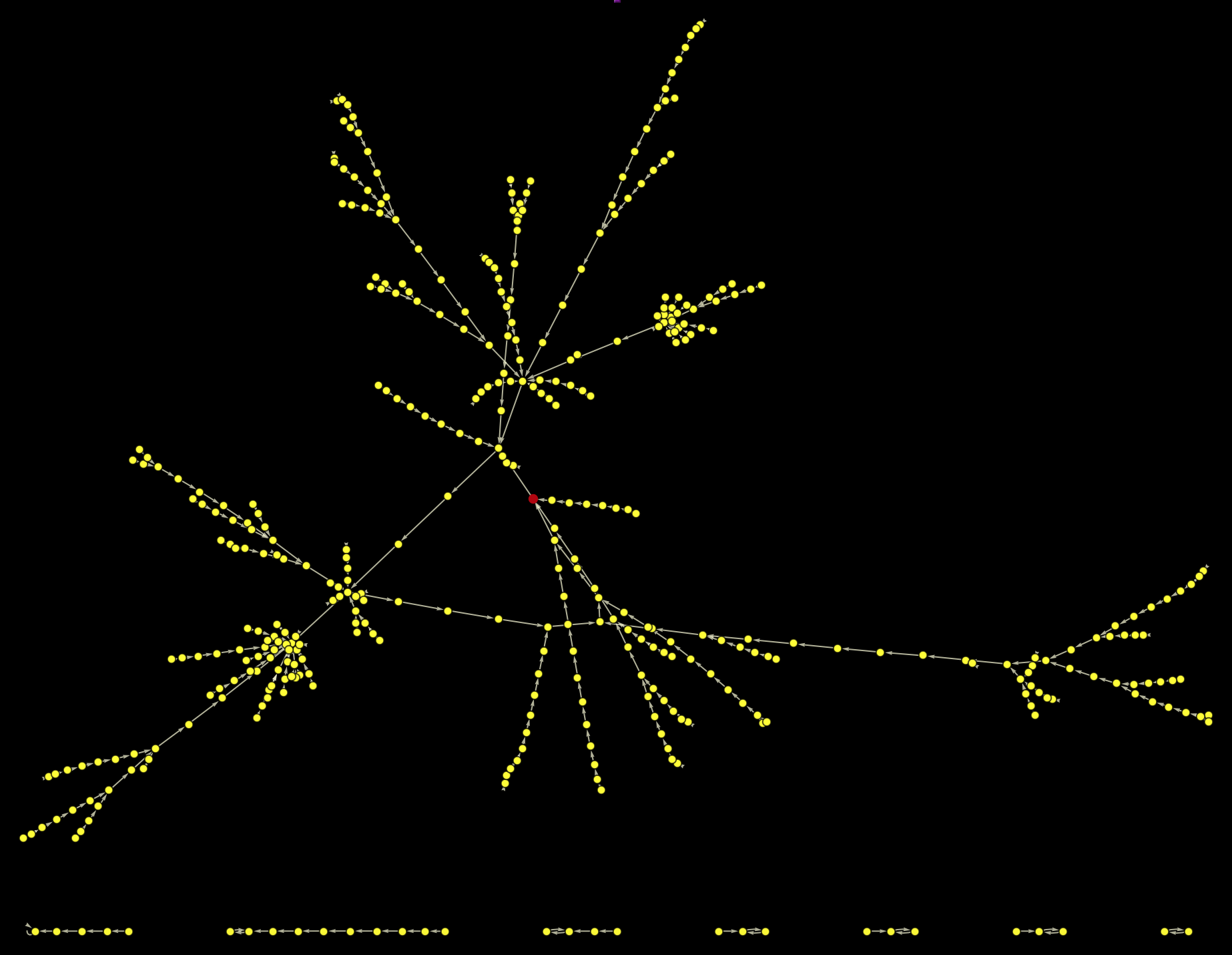
The red vertex represents the Philosophy article. It becomes clear that it is on a cycle - the same cycle we have observed for the case of Germany as initial page. If we remove the link from Philosophy to Greek_language we end up with images like these:
HighlightGraph[
 Graph[DeleteCases[DeleteDuplicates[
 Flatten[Rule @@@ Partition[StringDelete[#, "https://en.wikipedia.org/wiki/"], 2, 1] & /@ paths]], "Philosophy" -> "Greek_language"],
  Background -> Black, VertexStyle -> Yellow,
  EdgeStyle -> LightYellow, VertexSize -> 2, ImageSize -> Full,
  GraphLayout -> "RadialEmbedding"], "Philosophy"]
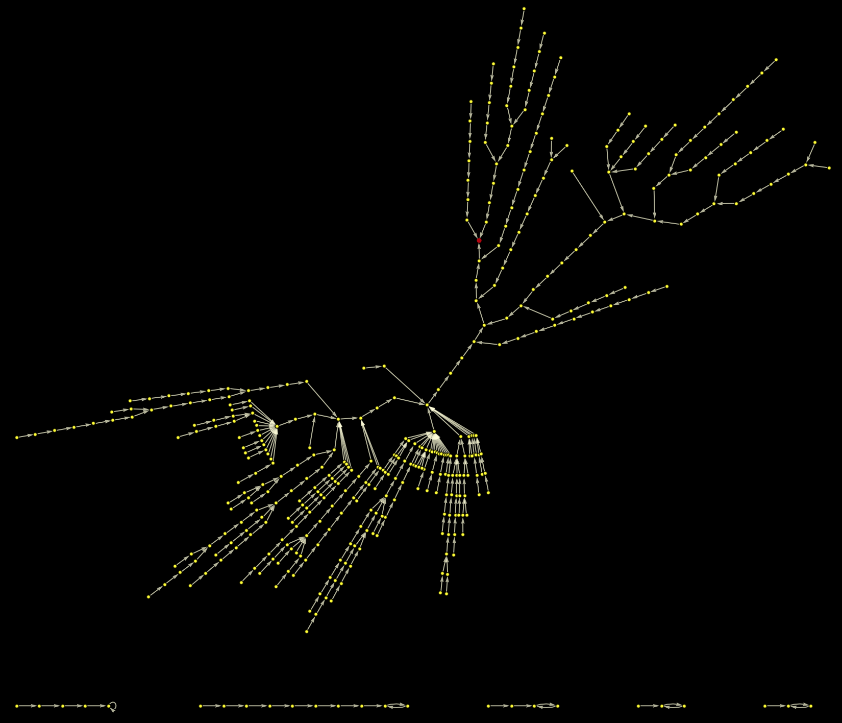
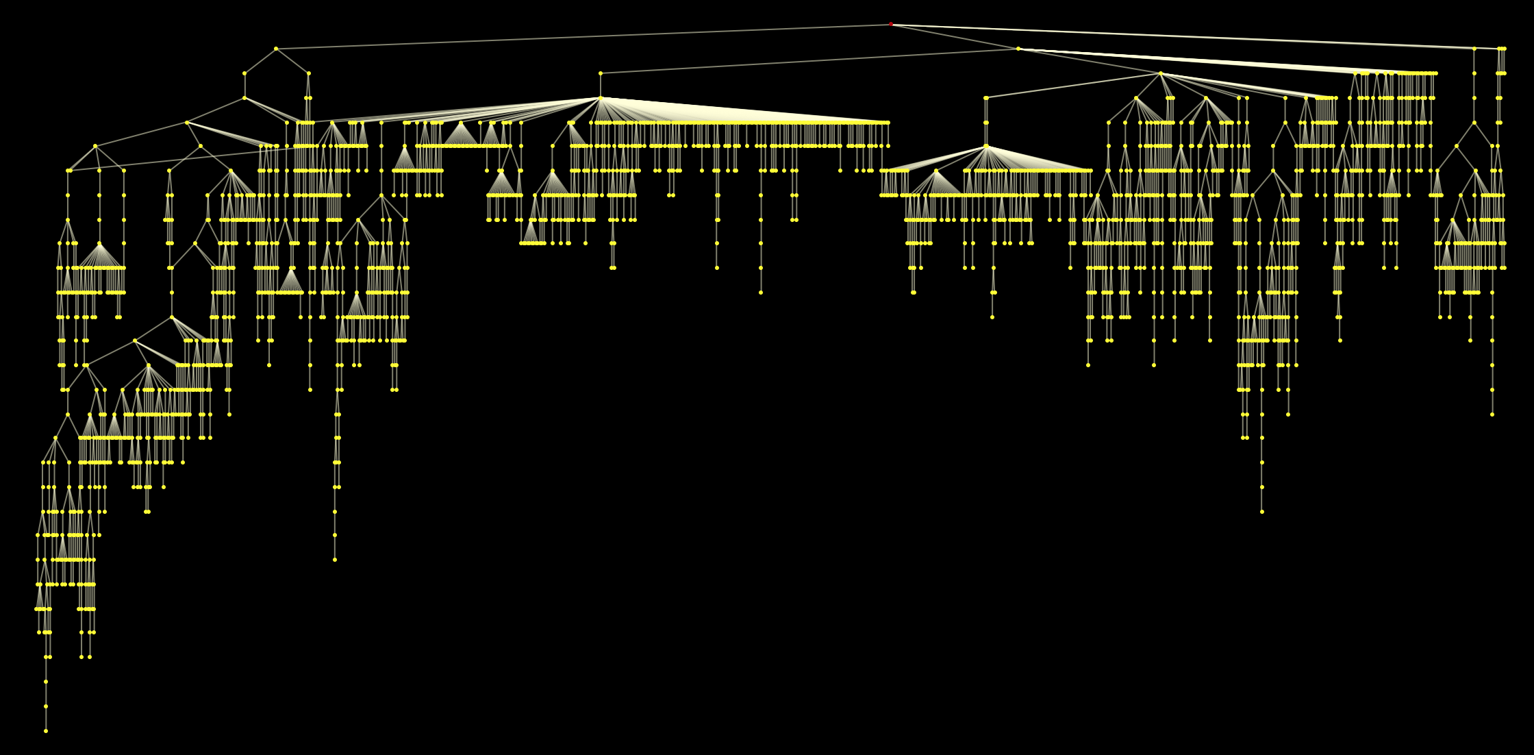
All paths on the largest component of the graph end up at the red point. Plotting this as a rooted graph makes the structure a bit clearer:
HighlightGraph[Graph[WeaklyConnectedGraphComponents[Graph[DeleteCases[DeleteDuplicates[Flatten[Rule @@@
Partition[StringDelete[#, "https://en.wikipedia.org/wiki/"], 2, 1] & /@ paths]], "Philosophy" -> "Greek_language"]]][[1]],
Background -> Black, VertexStyle -> Yellow, EdgeStyle -> LightYellow, VertexSize -> 0.4, ImageSize -> Full,
GraphLayout -> {"LayeredEmbedding", "RootVertex" -> "Philosophy"}], "Philosophy"]
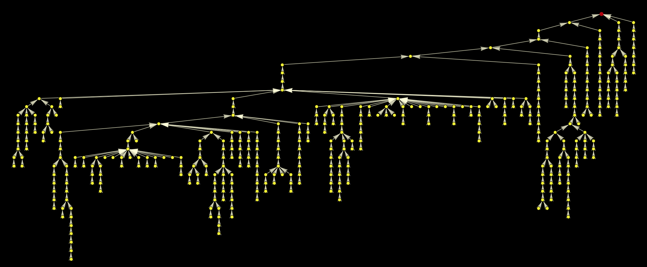
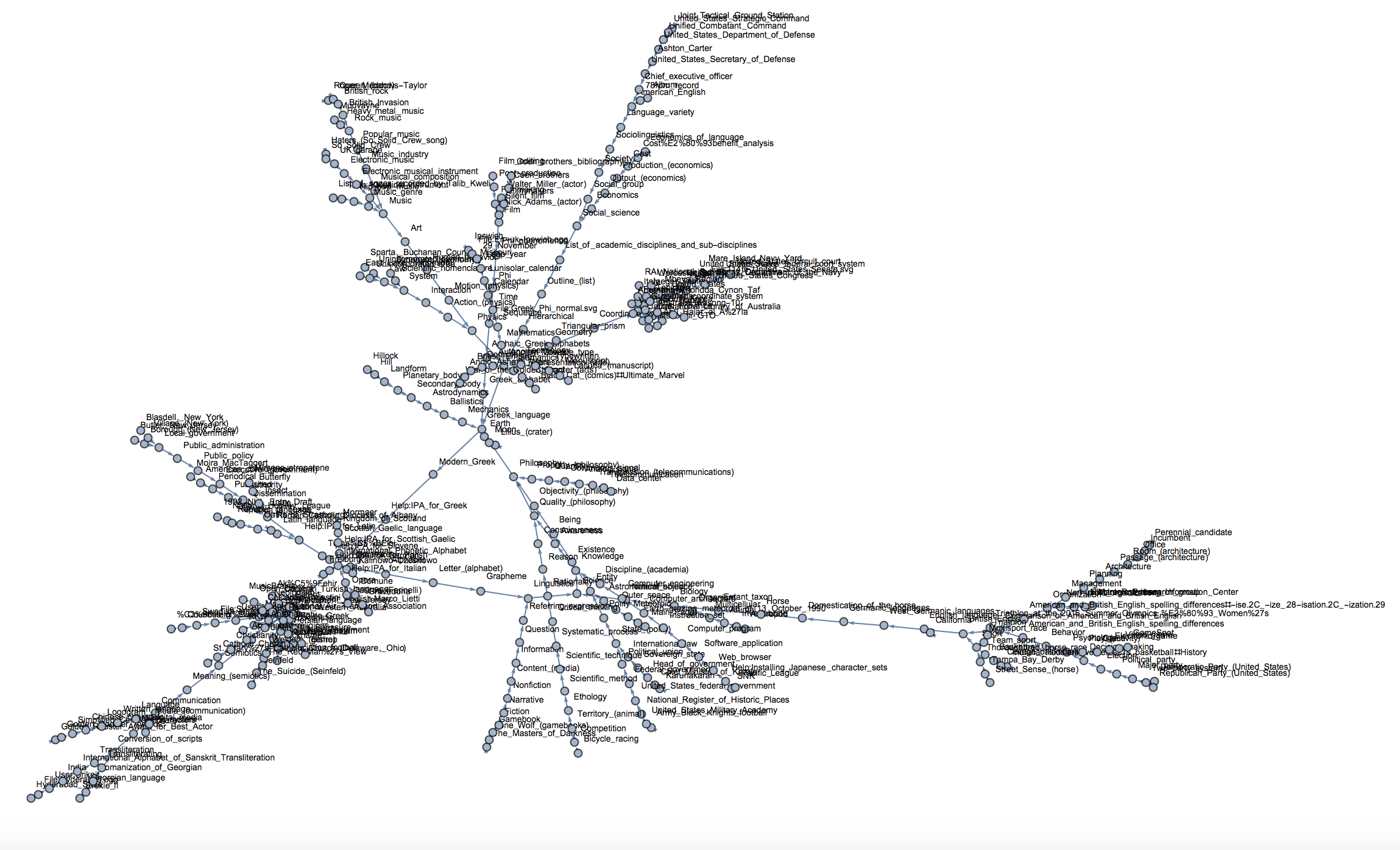
We can of course label the nodes, but this overloads the image somewhat:
Graph[DeleteDuplicates[Flatten[Rule @@@ Partition[StringDelete[#, "https://en.wikipedia.org/wiki/"], 2, 1] & /@ paths]], VertexLabels -> "Name",
VertexLabelStyle -> Directive[7], VertexSize -> 2, ImageSize -> Full]
Here's a 3D version:
Graph3D[DeleteDuplicates[Flatten[Rule @@@ Partition[StringDelete[#, "https://en.wikipedia.org/wiki/"], 2, 1] & /@ paths]], VertexSize -> 2, ImageSize -> Full]
A more comprehensive dataset
For a slightly more detailed analysis I will need more starting wiki pages.
startingpages1000 =
  DeleteDuplicates[Table[RandomChoice[Select[Import["https://en.wikipedia.org/wiki/Special:Random",
  "Hyperlinks"], (StringContainsQ[#, "https://en.wikipedia.org/wiki/"] && ! StringContainsQ[StringDelete[#, "https://en.wikipedia.org/wiki/"], ":"]) &]], {1200}]];
The next function should only be run with an appropriate Pause between the calls - Be nice to Wikipedia! It is an absolutely brilliant resource for everyone.
Monitor[paths1000 =
   Table[NestWhileList[(Select[Table[Quiet[("https://en.wikipedia.org/wiki" <>
   StringSplit[StringSplit[StringSplit[#, "<p>"][[k]], "<a href=\"/wiki"][[2]], "\""][[1]])], {k, 2, 10}],
   StringQ[#] &][[1]] &@Import[#, "Source"]) &, startingpages1000[[m]], UnsameQ, All], {m, 1, Length[startingpages1000]}];, m]
The code will run for many hours or days if you choose a good waiting time between calls. Let's save that again:
Export["~/Desktop/startingpages1000.mx", startingpages1000];
Export["~/Desktop/paths1000.mx", paths1000];
Let's prepare the data for further analysis:
paths1000clean = (Select[Select[Select[#, StringQ], ! StringContainsQ[#, "wiki<a href="] &], (StringContainsQ[#, "https://en.wikipedia.org/wiki/"] && !
StringContainsQ[StringDelete[#, "https://en.wikipedia.org/wiki/"], ":"]) &]) & /@ paths1000;
Here's the resulting graph:
HighlightGraph[Graph[WeaklyConnectedGraphComponents[Graph[DeleteDuplicates[Flatten[(Rule @@@
Partition[StringDelete[#, "https://en.wikipedia.org/wiki/"], 2, 1]) & /@ paths1000clean]]]][[1]], VertexStyle -> Yellow,
EdgeStyle -> Yellow], Graph[(Rule @@@ Partition[StringDelete[startGermany, "https://en.wikipedia.org/wiki/"], 2,1])[[6 ;;]]], Background -> Black]

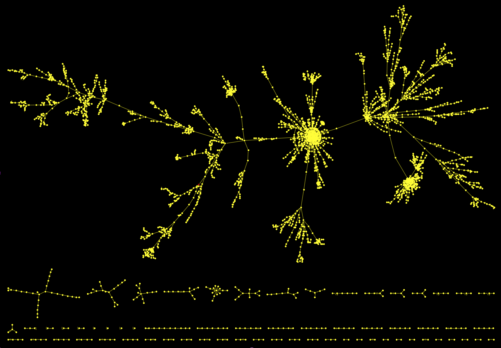
As a matter of fact, this is only the largest connected component of the graph. If we cut again the outgoing link from the Philosophy article and plot everything we get:
HighlightGraph[Graph[DeleteCases[DeleteDuplicates[Flatten[(Rule @@@
Partition[StringDelete[#, "https://en.wikipedia.org/wiki/"], 2, 1]) & /@ paths1000clean]], "Philosophy" -> "Greek_language"], ImageSize -> Full,
Background -> Black, EdgeStyle -> Yellow, VertexStyle -> Yellow], "Philosophy"]
We have
Length[paths1000]
1073 starting pages and there are
Length[WeaklyConnectedComponents[Graph[DeleteCases[DeleteDuplicates[Flatten[(Rule @@@
Partition[StringDelete[#, "https://en.wikipedia.org/wiki/"],2, 1]) & /@ paths1000clean]], "Philosophy" -> "Greek_language"], ImageSize -> Full,
Background -> Black, EdgeStyle -> Yellow, VertexStyle -> Yellow]]]
65 weakly connected components. This allows us to estimate (it is actually not the true value) that about
(1073 - 64)/1073.
or 94% of all websites lead to the Philosophy article, which is in relatively good agreement with the data on this website, where they obtain 97% - the difference might be in part due to my crude parsing and also because I use slightly different rules than they do. Also, I only use only a very small subset of all 5 million plus pages. Nevertheless, there is evidence for a large attractor.
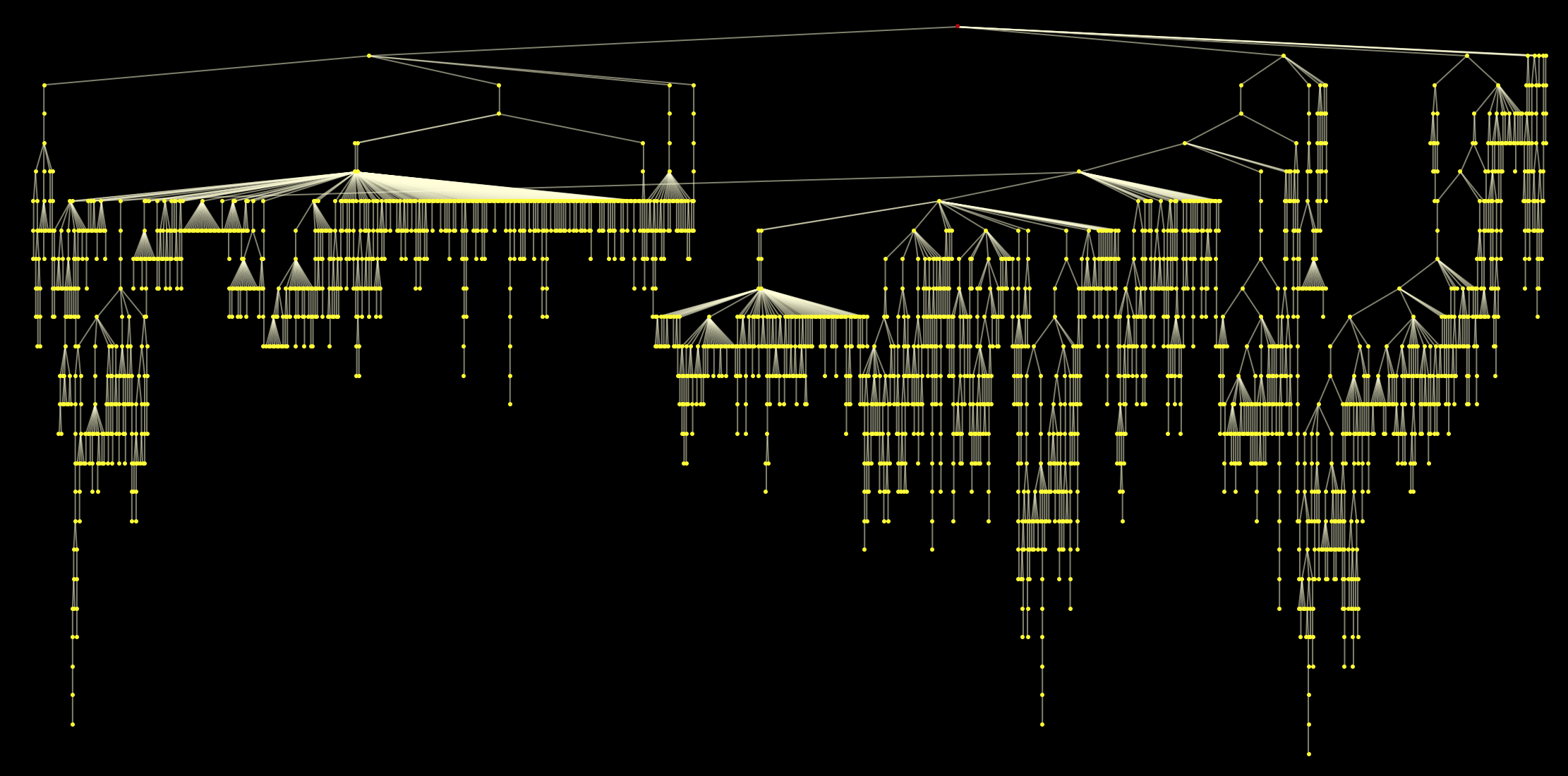
HighlightGraph[Graph[WeaklyConnectedGraphComponents[Graph[DeleteCases[DeleteDuplicates[Flatten[(UndirectedEdge @@@
Partition[StringDelete[#, "https://en.wikipedia.org/wiki/"], 2, 1]) & /@ paths1000clean]], "Philosophy" -> "Greek_language"]]][[1]], Background -> Black,
VertexStyle -> Yellow, EdgeStyle -> LightYellow, VertexSize -> 0.1, ImageSize -> Full, GraphLayout -> {"LayeredEmbedding", "RootVertex" -> "Philosophy"}], "Philosophy", ImagePadding -> 10, AspectRatio -> 1/2]
Note that we could of course take any other page on our attractor
Graph[(Rule @@@ Partition[StringDelete[startGermany, "https://en.wikipedia.org/wiki/"], 2, 1])[[6 ;;]], VertexLabels -> Placed["Name", Above],
 VertexStyle -> Yellow, EdgeStyle -> Yellow, VertexLabelStyle -> Directive[Yellow, 20], Background -> Black]
as the target state. But it sounds much nicer to claim that the greatest collection of human knowledge all leads to Philosophy. If you were inclined to do so you could also claim that it leads to the "international phonetic alphabet" or to "science". I have a tendency for the latter and therefore want to add the respective graph plot:
HighlightGraph[Graph[WeaklyConnectedGraphComponents[Graph[DeleteCases[DeleteDuplicates[Flatten[(UndirectedEdge @@@
Partition[StringDelete[#, "https://en.wikipedia.org/wiki/"], 2, 1]) & /@ paths1000clean]], "Science" -> "Knowledge"]]][[1]], Background -> Black,
VertexStyle -> Yellow, EdgeStyle -> LightYellow, VertexSize -> 0.1, ImageSize -> Full, GraphLayout -> {"LayeredEmbedding", "RootVertex" -> "Science"}], "Science", ImagePadding -> 10, AspectRatio -> 1/2]
Some basic characteristics of the network
We can now also make some simple calculations about properties of these graphs. First we try to find out which node represents the Philosophy article:
Position[VertexList[WeaklyConnectedGraphComponents[Graph[DeleteCases[DeleteDuplicates[Flatten[(Rule @@@
Partition[StringDelete[#, "https://en.wikipedia.org/wiki/"], 2, 1]) & /@ paths1000clean]], "Philosophy" -> "Greek_language"]]][[1]]], "Philosophy"]
which gives 320. Next we can calculate the distance matrix between all nodes:
distmatrix =
  GraphDistanceMatrix[WeaklyConnectedGraphComponents[Graph[DeleteCases[DeleteDuplicates[Flatten[(Rule @@@
  Partition[StringDelete[#, "https://en.wikipedia.org/wiki/"], 2, 1]) & /@ paths1000clean]], "Philosophy" -> "Greek_language"]]][[1]]];
and check the distance of all other articles to the Philosophy article:
dist2philosophy = Transpose[distmatrix][[320]];
What's the mean path length?
N@Mean[dist2philosophy]
which gives 14.6.
The median
N@Median[dist2philosophy]
is 15. These values are lower than the ones reported on the page above, which gives a median length of 23. We can also plot a histogram
Histogram[dist2philosophy, PlotTheme -> "Marketing", FrameLabel -> {"Path length", "Number of paths"},
 LabelStyle -> Directive[Bold, Medium], ChartStyle -> Red, ImageSize -> Large]
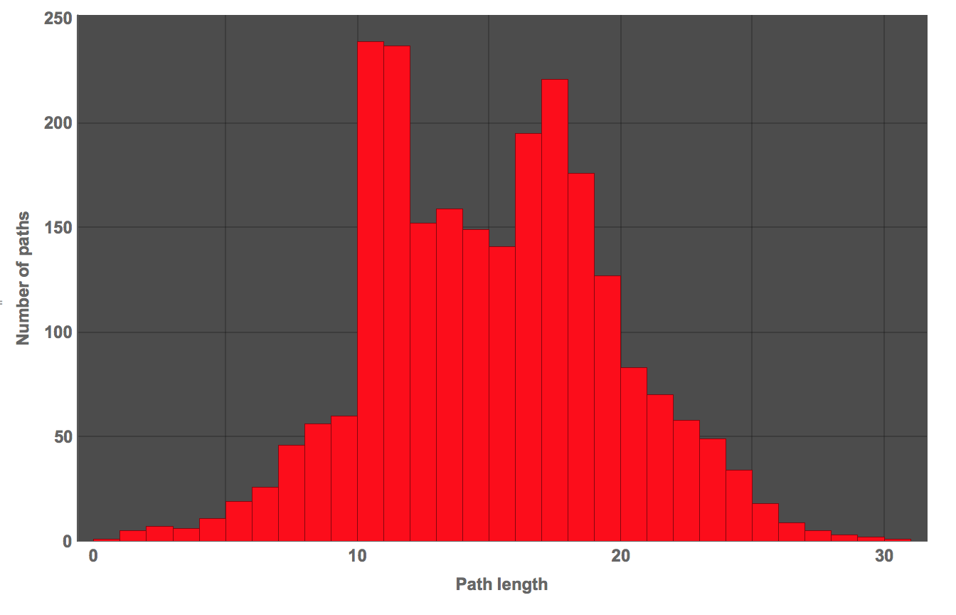
Well, this is not too bad, but it does not seem to correspond perfectly to what is reported either. I do use slightly different rules though. I am currently working on a much more efficient way of doing this with the Wolfram Language. If it works I might post it later.
Disclaimer & what to do if you want to reproduce that
Note, that you should not run the crawler without a delay between consecutive requests. To allow you to run the code, I will add the files with the data I have downloaded.
Discussion
The explanation for this curious structure of the nearly global attractor is still not quite clear. There are hypothesis such as the fact that authors are encouraged to start an article by a definition of the topic of the article. This might lead to a sort of classification chain which ends up at areas such as Philosophy and Science. Differently from the standard procedure my paring does maintain links to the phonetical transcription. What is interesting is that in spite of several differences between my and the standard procedure the main effect of ending up at Philosophy (or Science) is still there and hence appears to be robust with respect to smaller changes in the algorithm - and that's quite cool.
Cheers,
Marco
 Attachments:


