Message Boards Message Boards

0
|
4466 Views
|
2 Replies
|
1 Total Likes
View groups...
Share
Share this post:

Avoid NDSolve issue with boundary conditions?

The code

x0 = 0.25;  T = 20;   u1 = -0.03;  u2 = 0.07;  u3 = -0.04;
a = 1/100;   t0 = 5;  omega = 2;
a = 0.01;  dis[x_] := a/(Pi (x^2 + a^2))
P[t_] := If[t <= t0, Sin[omega t], 0]
u[t_] := u1 HeavisideTheta[t - 0.8] + 
  u2 HeavisideTheta[t - 1.64] + u3 HeavisideTheta[t - 3.33]

pde = a D[w[x, t], {x, 4}] + D[w[x, t], {t, 2}] - 
   P[t] dis[x - x0];
sol = NDSolve[{pde == 0, w[0, t] == u[t], w[1, t] == 0, 
    Derivative[2, 0][w][0, t] == 0, Derivative[2, 0][w][1, t] == 0, 
    w[x, 0] == 0, Derivative[0, 1][w][x, 0] == 0}, 
   w[x, t], {x, 0, 1}, {t, 0, 80}, Method -> "StiffnessSwitching"];

gives an error

NDSolve::eerr: Warning: scaled local spatial error estimate of 246.5944594961422` at t = 80.` in the direction of independent variable x is much greater than the prescribed error tolerance. Grid spacing with 25 points may be too large to achieve the desired accuracy or precision. A singularity may have formed or a smaller grid spacing can be specified using the MaxStepSize or MinPoints method options.

I think it`s because of the boundary conditions on derivatives. Have tried Automatic, MethodOfLines, etc., does not help. Tried

Method -> {"MethodOfLines", 
      "SpatialDiscretization" -> {"TensorProductGrid", 
        "MinPoints" -> 100}}

works fine with second order equation subjected to bc containing only first order derivative. Any thoughts, hints?

2 Replies

Thank you very much! Oscillations, occurring in the solution for 0<t<20 (say) are very suspicious, the solution actually is a "very" smooth function.

This is no error only, a warning messages.

How about:

x0 = 0.25;  T = 20;   u1 = -0.03;  u2 = 0.07;  u3 = -0.04;
a = 1/100;   t0 = 5;  omega = 2;
a = 0.01;  dis[x_] := a/(Pi (x^2 + a^2))
P[t_] := If[t <= t0, Sin[omega t], 0]
u[t_] := u1 HeavisideTheta[t - 0.8] + 
  u2 HeavisideTheta[t - 1.64] + u3 HeavisideTheta[t - 3.33]

pde = a D[w[x, t], {x, 4}] + D[w[x, t], {t, 2}] - 
   P[t] dis[x - x0];

ppR = 50;(* for better result you can increase this number . Beware, more RAM and CPU time *)

sol = NDSolve[{pde == 0, w[0, t] == u[t], w[1, t] == 0, 
    Derivative[2, 0][w][0, t] == 0, Derivative[2, 0][w][1, t] == 0, 
    w[x, 0] == 0, Derivative[0, 1][w][x, 0] == 0}, 
   w[x, t], {x, 0, 1}, {t, 0, 80}, 
MaxSteps -> Infinity, 
PrecisionGoal -> 2,
AccuracyGoal -> 2, 
Method -> {"MethodOfLines", 
     "SpatialDiscretization" -> {"TensorProductGrid", "MinPoints" -> ppR,
        "MaxPoints" -> ppR, "DifferenceOrder" -> 2}, 
     Method -> {"Adams", "MaxDifferenceOrder" -> 1}}];

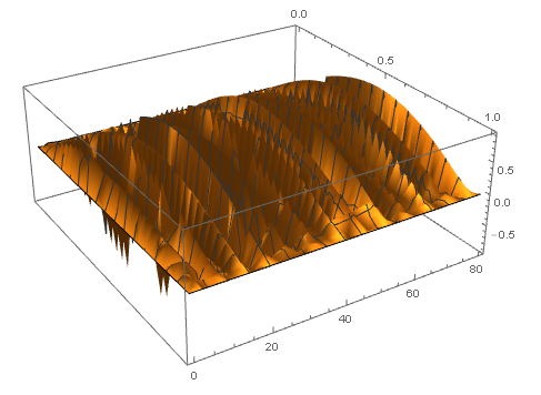
Plot3D[Evaluate[w[x, t] /. sol], {x, 0, 1}, {t, 0, 80}]

enter image description here

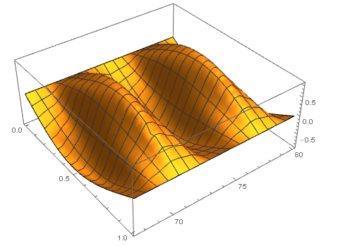
Plot3D[Evaluate[w[x, t] /. sol], {x, 0, 1}, {t, 80 - 4*Pi, 80}]

enter image description here

POSTED BY: Mariusz Iwaniuk
Reply to this discussion
Community posts can be styled and formatted using the Markdown syntax.
Reply Preview
Attachments
Remove
or Discard

Group Abstract Group Abstract