Message Boards Message Boards

Root plotting function from Paul Wellin's book?

Posted 8 years ago

In An introduction to programming with Mathematica by Paul R. Wellin, Richard J. Gaylord, Samuel N. Kamin, there is a section in page 279 that about root finding with this code:

RootPlot[fun_, {x_, xmin_, xmax_}] := 
 Module[{z, fplot, pts, spts, roots, points, 
   f = Function[{x, Evaluate[fun]}]}, 
  fplot = Plot [f [x], {x, xmin, xmax}, DisplayFunction -> Identity]; 
  pts = Cases[fplot, Line[{ z__ }] -> z, Infinity]; 
  spts = Map[First, 
    Select[Split[pts, Sign[Last[# 2]] == -Sign[Last[# 1]] &], 
     Length[# 1] == 2 &], {2}]; 
  roots = Map[FindRoot[f[x] == 0, {x, # [[ 1]], # [[2]]}] &, spts]; 
  points = Map[Point[{#, 0}] &, x /. roots]; 
  Show[fplot, DisplayFunction -> $DisplayFunction, 
   Epilog -> {RGBColor[ 0, 0, 1], PointSize[.02], points}]; roots]

Actually when i made an effort to test this code for Sin[2x] something happened wrong! Please check it out and tell what is mistake!?

POSTED BY: Hadi Tokme
5 Replies

Not sure if this is really relevant, but you should look this up. Sharing my solution:

FindCrossings2D[{f_, g_}, {x_, xmin_, xmax_}, {y_, ymin_, ymax_}] := 
  {x, y} /. (FindRoot[{f[x, y] == 0, g[x, y] == 0}, {{x, #[[1]]}, 
  {y, #[[2]]}}] & /@ (ContourPlot[{f[x, y] == 0, g[x, y] == 0}, 
  {x, xmin, xmax}, {y, ymin, ymax}][[1, 1]]))

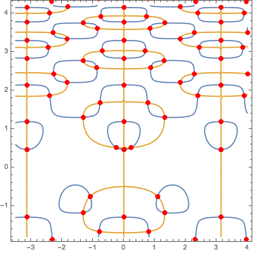
f[x_, y_] := -Cos[y] + 2 y Cos[y^2] Cos[2 x];
g[x_, y_] := -Sin[x] + 2 Sin[y^2] Sin[2 x];

pts = FindCrossings2D[{f, g}, {x, -7/2, 4}, {y, -9/5, 21/5}];

ContourPlot[{f[x, y] == 0, g[x, y] == 0}, {x, -7/2, 4}, {y, -9/5, 21/5},
 Epilog -> {AbsolutePointSize[6], Red, Point /@ pts}]

enter image description here

POSTED BY: Vitaliy Kaurov
Posted 8 years ago

Vitaliy, you are right but here FindCrossing2D will take two equations,f and g, and return all the simultaneous solutions (only the crossings!). My question was about when we have only one function such as f(x,y)!! can we put zero instead of g(x,y)?

POSTED BY: Hadi Tokme
Posted 8 years ago

After clearing this algorithm, now there is one question: How can we rewrite this algorithm for Contour plot with two variables?

POSTED BY: Hadi Tokme
Posted 8 years ago

Great!...thanks. This method can be very useful to solve Transcendental equations.

POSTED BY: Hadi Tokme

There must not be a space between # and the numbers 1 or 2. Then the plot code should be updated from the version 5 style:

RootPlot[fun_, {x_, xmin_, xmax_}] :=

 Module[{z, fplot, pts, roots, spts, points,
   f = Function @@ {x, fun}},
  fplot = Plot[fun, {x, xmin, xmax}];
  pts = Cases[fplot, Line[{z__}] -> z, All];
  spts = Map[First, 
    Select[Split[pts, Sign[Last[#2]] == -Sign[Last[#1]] &], 
     Length[#1] == 2 &], {2}];
  roots = Map[FindRoot[f[x] == 0, {x, #[[1]], #[[2]]}] &, spts];
  points = Map[Point[{#, 0}] &, x /. roots];
  Print@Show[fplot, 
    Epilog -> {Blue, PointSize[.02], points}];
  roots]

It works for me now:

RootPlot[Sin[2 x], {x, 0, 3 Pi}]

enter image description here

POSTED BY: Gianluca Gorni
Reply to this discussion
Community posts can be styled and formatted using the Markdown syntax.
Reply Preview
Attachments
Remove
or Discard

Group Abstract Group Abstract