SUPPLEMENTARY WOLFRAM MATERIALS for ARTICLE:

Mias, G., Yusufaly, T., Roushangar, R. et al.

MathIOmica: An Integrative Platform for Dynamic Omics. Sci Rep 6, 37237 (2016).

NATURE Scientific Reports

https://doi.org/10.1038/srep37237

Introduction: MathIOmica

My lab has recently released a new package for Mathematica, focusing on bioinformatics: MathIOmica (mathiomica.org, download at GitHub). The package is released under an MIT License and is available to use for free (requires Mathematica 10.4+).

Background

There has been ongoing effort on the analysis of multiple omics data from disparate biological sources. Multimodal data from various sources in now available, particularly with new enabling technologies under constant development (e.g. sequencing capabilities with next generation sequencing and the focus on transcriptomics, i.e. the set of all transcripts (RNA) in a cell, or mass spectrometry use for proteomics, i.e. the set of all proteins in a cell). The recently announced Precision Medicine Initiative will lead to more being produced in the next few years. This has led to the development of multiple bioinformatics tools and platforms, particularly for R and Python, such as Bioconductor and Biopython aiming to integrate information from various omics, including in the context of personalized medicine (Mias and Snyder, 2014). However, sophisticated mathematical methods to study the dynamics of omics data are still underdeveloped, particularly methods that address missing data and uneven sampling over time, as well as time-series classifications.

Implementation

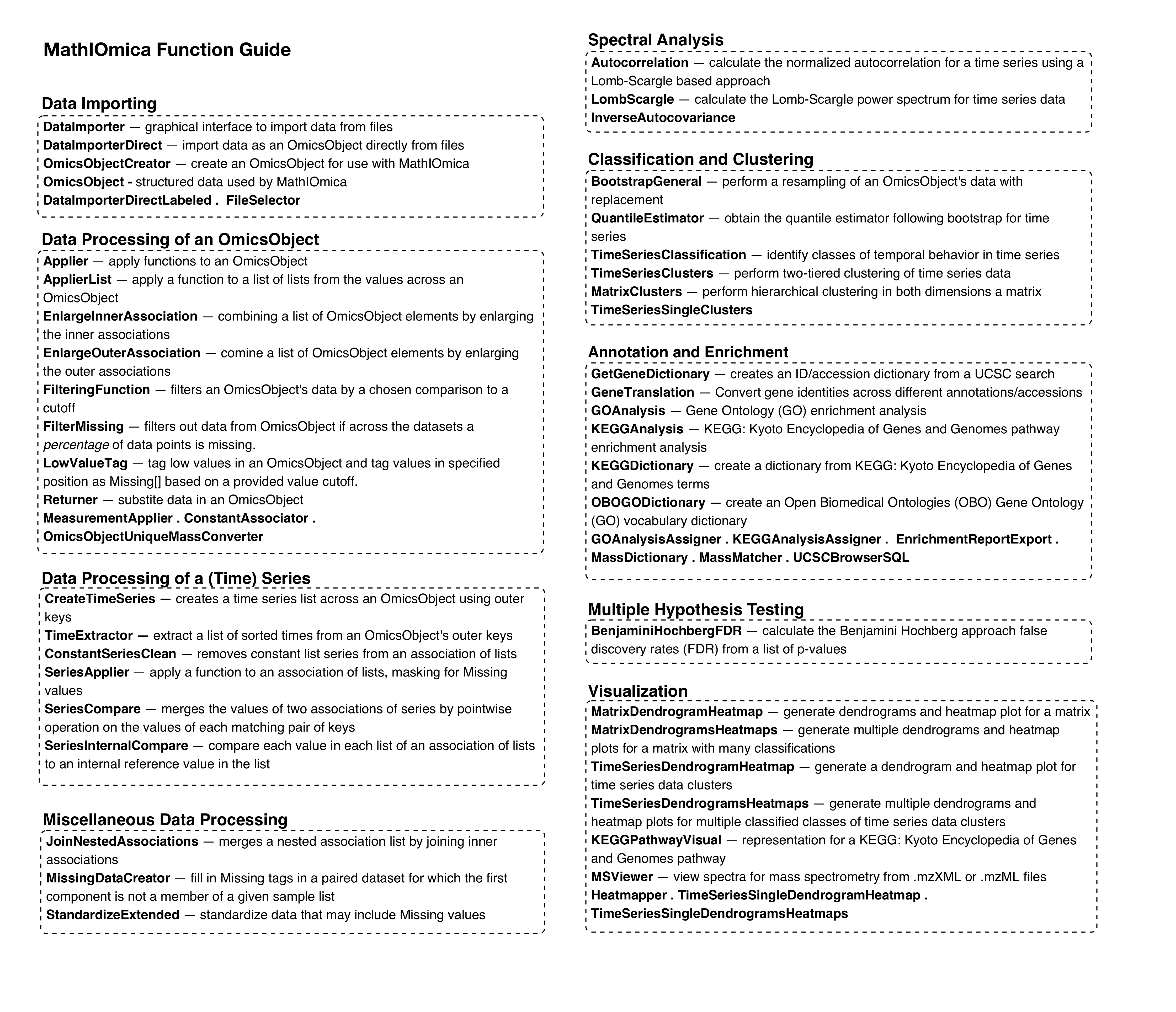
Coming from a physics background and transitioning to genetics, I decided I wanted to develop a bioinformatics package for Mathematica written in the Wolfram Language. The MathIOmica package particularly focuses on the integration of multiple omics information from dynamic profiling in a personalized medicine profiling approach. Additionally, it provides essential functions to facilitate general bioinformatics analysis in Mathematica. This includes data importing and preprocessing, including normalizations, and clustering and visualization of the classification of dynamic data. MathIOmica includes annotations from Gene Ontology, as well as KEGG pathway analyses. MathIOmica was built using Wolfram Workbench and includes inbuilt documentation accessible within Mathematica after installation. This first release is a first step, in which we wanted to develop a base for bioinformatics tools in the Wolfram Language and we are now working on more advanced functionality. The main functionality is summarized below (Figure from Mias et. al, 2016).

Example Using Transcriptome Data

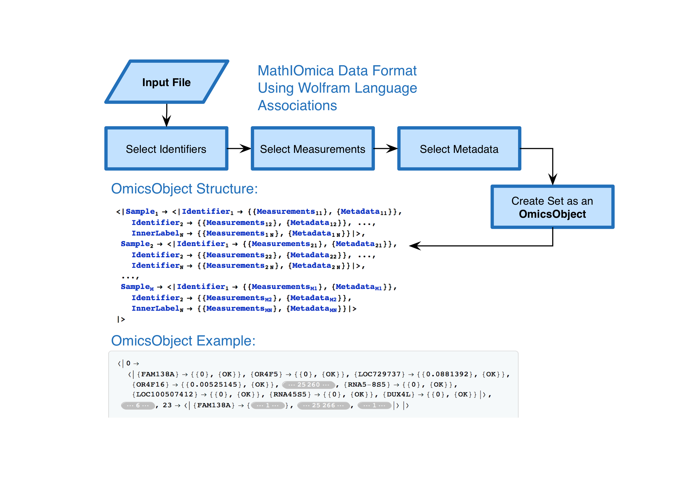
MathIOmica is meant to be used for biological data. Typically such data contains measurements, but also metadata. Additionally, multiple samples may be available. To parse such data we decided to create an OmicsObject, essentially an association of associations (Figure From from Mias et. al, 2016):

Multiple utilities exist within the package to create and handle OmicsObjects, and many examples. Here let us take a close look at an example using transcriptomics data from a pilot first integrative Personal Omics Profiling (iPOP) project as an implementation of using MathIOmica to look at dynamics of biological data. This study was meant as a prototype to observe the personal omics dynamics from a single person, including proteomics transcriptomics and metabolomics profiled from blood. Different samples (from 7 to 21 included here) were obtained at different time points. The time points included here correspond to days ranging from 186th to the 400th day of the study, (this can be represented in the following sample to day association:

<|7->186,8->255,9->289,10->290,11->292,12->294,13->297,14->301, 15->307,16->311,17->322,18->329,19->369,20->380,21->400|>.

On day 289 the subject of the study had a respiratory syncytial virus infection. Additionally, after day 301, the subject displayed high glucose levels and was eventually diagnosed with type 2 diabetes. All these data are included as part of MathIOmica's examples.

We first load the package (assuming it has been installed):

<<`MathIOmica`

Then we can load the OmicsObject associated with the transcriptome data:

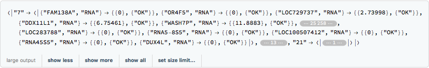
rnaExample = 
 Get[FileNameJoin[{ConstantMathIOmicaExamplesDirectory, 
    "rnaExample"}]]

The outer keys correspond to the sample enumeration for a given day. We can convert these to actual days of the study and use KeyMap to change the outer labels:

sampleToDays = <|"7" -> "186", "8" -> "255", "9" -> "289", 
   "10" -> "290", "11" -> "292", "12" -> "294", "13" -> "297", 
   "14" -> "301", "15" -> "307", "16" -> "311", "17" -> "322", 
   "18" -> "329", "19" -> "369", "20" -> "380", "21" -> "400"|>;

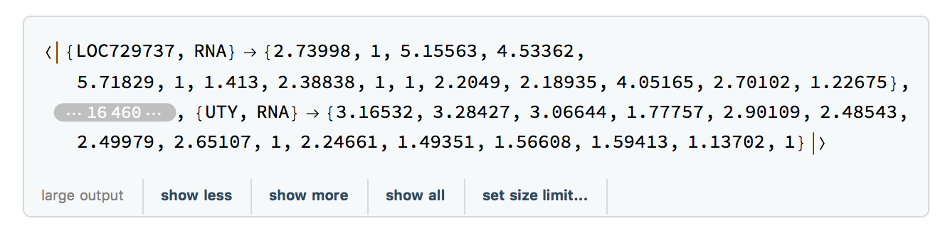
rnaLongitudinal = KeyMap[sampleToDays, rnaExample]

Next, we can normalize our dataset. The inner measurements to be normalized are actual FPKM values ( fragments per kilobase of transcript per million mapped reads). A typical normalization used for RNA-Sequencing (RNA-Seq) FPKMs from transcriptomes across multiple samples is quantile normalization.

rnaQuantileNormed = QuantileNormalization[rnaLongitudinal]

We additionally do some basic quality control as an example. First we set all FPKMs that are 0 to Missing, i.e. 0 means nothing was detected so that gene fragment is actually Missing.

rnaZeroTagged = LowValueTag[rnaQuantileNormed, 0]

We then want to account for noisy measurements. If we assume all values less than unity are essentially noise and indistinguishable, we set them all to unity:

rnaNoiseAdjusted = 
 LowValueTag[rnaZeroTagged, 1, ValueReplacement -> 1]

We then filter out data where the reference healthy point we want to compare against, which is day "255", is missing, and retain data with at least 3/4 of the points available :

rnaFiltered = FilterMissing[rnaNoiseAdjusted, 3/4, Reference -> "255"]

The following charts are generated that show the remaining points in the data, including the statistics for Missing tags: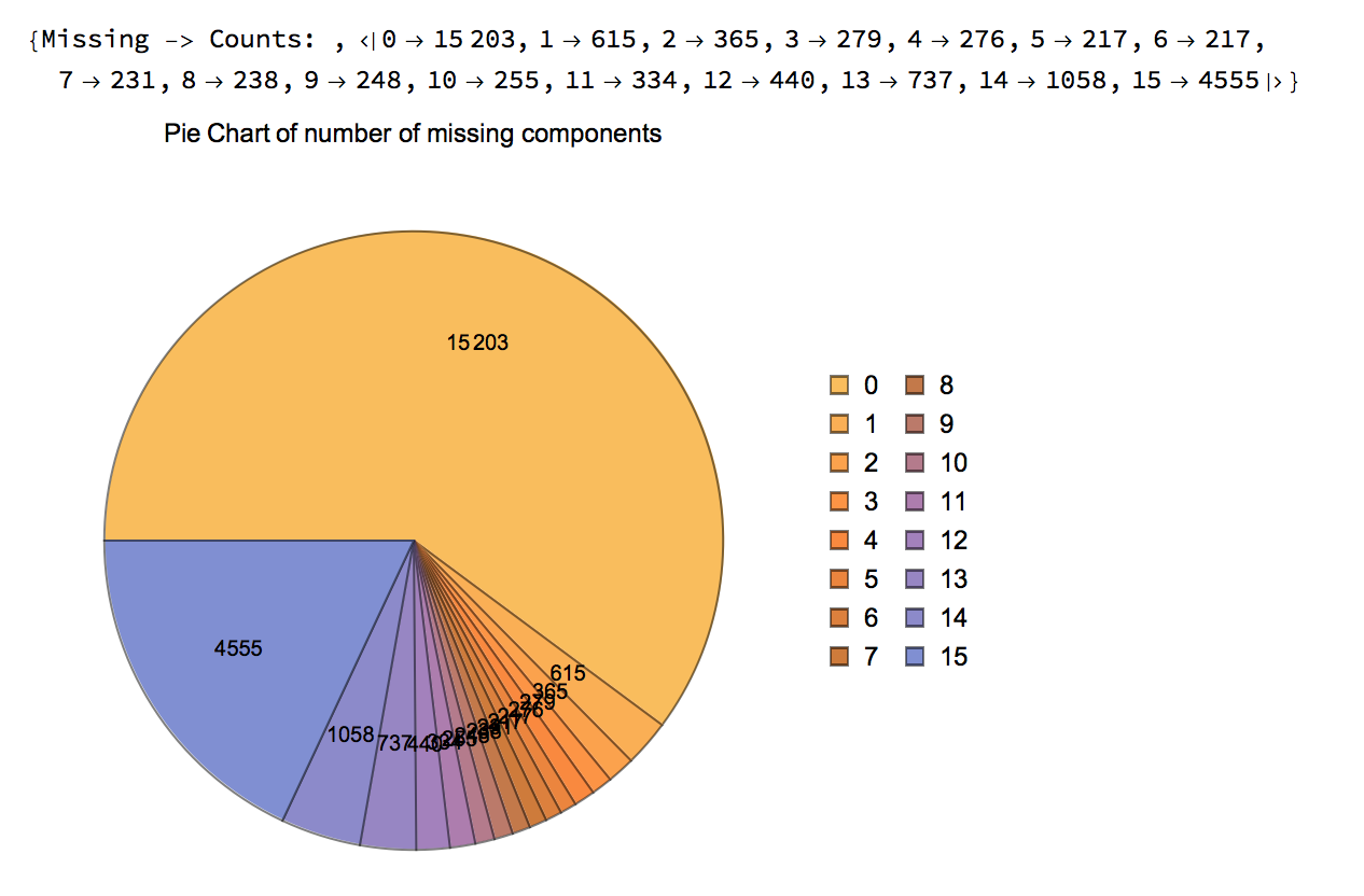

We extract the times for the filtered RNA data using:

timesRNA = TimeExtractor[rnaFiltered]

The result is timesRNA={186, 255, 289, 290, 292, 294, 297, 301, 307, 311, 322, 329, 369, 380, 400}, a list of the days on which samples were taken in the study.

For each gene we can now extract a time series (list of values) corresponding to these times:

timeSeriesRNA = CreateTimeSeries[rnaFiltered]

We would next like to identify temporal trends in the data. To do this we first want to create a resampled distribution for the transcriptome dataset prior to classification and clustering to be able to compare against random time series from the same type of data. We repeat the steps in the processing as described above using a resampled set of measurements. For brevity all steps (9) are listed together:

(*Bootstrap of 100000 time series*)
rnaBootstrap = BootstrapGeneral[rnaLongitudinal, 100000];
(*1: quantile normalization*)rnaBootstrapQuantileNormed = 
  QuantileNormalization[rnaBootstrap];
(*2: tag zero values*)rnaBootstrapZeroTagged = 
  LowValueTag[rnaBootstrapQuantileNormed, 0];
(*3: tag noise*) rnaBootstrapNoiseAdjusted = 
  LowValueTag[rnaBootstrapZeroTagged, 1, ValueReplacement -> 1];
(*4: filter missing*) rnaBootstrapFiltered = 
  FilterMissing[rnaBootstrapNoiseAdjusted, 3/4, Reference -> "255", 
   ShowPlots -> False];
(*5: create time series*) timeSeriesBootstrapRNA = 
  CreateTimeSeries[rnaBootstrapFiltered];
(*6: take log*) timeSeriesBootstrapRNALog = 
  SeriesApplier[Log, timeSeriesBootstrapRNA];
(*7: compare to reference healthy point*)rnaBootstrapCompared = 
  SeriesInternalCompare[timeSeriesBootstrapRNALog, 
   ComparisonIndex -> 2];
(*8: normalize series*)normedBootstrapRNACompared = 
  SeriesApplier[Normalize, rnaBootstrapCompared];
(*9: remove constant series*)rnaBootstrapFinalTimeSeries = 
  ConstantSeriesClean[normedBootstrapRNACompared];

Now we have the random distribution we can proceed with classification. We want to classify the temporal behavior of genes to identify common trends. This is done by the provided TimeSeriesClassification function. The function uses a few methods to help classify time series with uneven time sampling, and in this example we will use an approach that computes internally a Lomb-Scargle periodogram. Classification is then based on periodograms, and the data is classified into classes of major (highest intensity) frequencies and spikes (maxima or minima in real signal intensity), depending on cutoffs typically provided by simulation.

Specifically, for a given signal $X_ j$, with length $N$, we have $N$ time measurements, namely $X_j=\left\{X_j\left(t_1\right),X_j\left(t_2\right),\text{...},X_j\left(t_N\right)\right\}$and can calculate the signal's periodogram (Lomb-Scargle method). The TimeSeriesClassification function uses the n=Floor[N/2] frequencies, $f_j=\left\{ f_{\text{j1}},f_{\text{j2}},\text{...},f_{\text{jk}},\text{...},f_{\text{jn}} \right\}$ and obtains corresponding n intensities, $I_j=\left\{I_{\text{j1}},I_{\text{j2}},\text{...},I_{\text{jn}}\right\}$. The default functionality is for $I_j$ to be calculated as a normalized vector. The maximum intensity of this vector, $I_{jk_{\text max}}=\text{Max}\left[I_j\right]$ corresponds to a dominant frequency $f_{jk_{\text max}}$, and occurs at some index $k_{\text max}$. For each signal $X_j$ we can then compare $I_{jk_{\text max}}$ to a cutoff intensity $I_{\text cutoff}$ to see if $I_{jk_{\text max}} > I_{\text cutoff}$. If so, the signal is placed in class $f_{k_{\text max}}$. A maximum of n classes is thus possible, and possible classes are labeled as $\left\{f_1,f_2,\text{...},f_k,\text{...},f_n\right\}$. The exact frequency list will depend on n, and hence the length of the input set times N, and is determined automatically by the classification functions.

Signals that do not show a maximum intensity in frequency space above the cutoff intensity,i.e. signals $j$ for which $I_{ j k} \le I_{\text cutoff}$ for all $k$, are checked for sudden signal spikes at any time point,and if so classified as spike maxima or minima. For each signal not showing a maximum periodogram intensity, $\tilde{X_j}$, we can calculate the real signal maximum, $\text{max}_j=\text{Max}\left[\tilde{X_j}\right]$,and minimum $\text{min}_ j=\text{Min}\left[\tilde{X_j}\right]$, from signal intensities across all time points. We can compare these values against cutoffs $\left\{\text{Minimum Spike Cutoff}_n, \text{Maximum Spike Cutoff}_n\right\}$provided by the user: These cutoffs are dependent on the length of a time series, $n$, and typically would correspond to the 95th quantile of distributions of maxima and minima of randomly generated signals.These cutoff values are provided by the SpikeCutoffs option value for each length $n$ involved in the computation as part of an association for different lengths: $<|\ ..., n\rightarrow \{\text {Minimum Spike Cutoff}_n,\text{Maximum Spike Cutoff}_n\},\ ...,\\ \text{length } i\rightarrow \{\text{Minimum Spike Cutoff}_i,\text{Maximum Spike Cutoff}_ i\},...|>$.

If a signal of length $n$, $\tilde{X_j}$, has $\text{max}_j > \text{Maximum Spike Cutoff}_n$, it is classified in the "SpikeMax" class, or otherwise if a signal $\tilde{X_j}$ has $\text{min}_ j < \text{Minimum Spike Cutoff}_n$, it is classified in the "SpikeMin" class. Signals for which the maximum signal intensity is not above the cutoffs are not reported.

The default output for this "Lomb-Scargle" method by the TimeSeriesClassification function is an Association with outer keys being the classification classes $C$,where $C\in \left\{f_1,f_2,\text{...},f_k,\text{...},f_n,\ \text{SpikeMax},\text{ SpikeMin}\right\} $, inner keys being the class members,Subscript[signalsX, j],and each class member value being a list of $\{\{\text{periodogram intensity list for signal }X_j\}, \{\text{input data list for }X_j\}\}$.

Before we classify our transcriptome data, we estimate for the "LombScargle" Method a 0.95 quantile cutoff from the bootstrap transcriptome data:

q95RNA = 
 QuantileEstimator[rnaBootstrapFinalTimeSeries, timesRNA] (*~0.85766 - this will vary depending on the simulation realization*)

Next, we estimate the "Spikes" 0.95 quantile cutoff from the bootstrap transcriptome data :

q95RNASpikes = 
 QuantileEstimator[rnaBootstrapFinalTimeSeries, timesRNA, 
  Method -> "Spikes"]
(*<|12 -> {0.817567, -0.441325}, 13 -> {0.803445, -0.423142}, 
 14 -> {0.782053, -0.409893}, 15 -> {0.762132, -0.374392}|> This will also vary depending on the simulation realization*)

Now we can classify the transcriptome time series data based on these cutoffs:

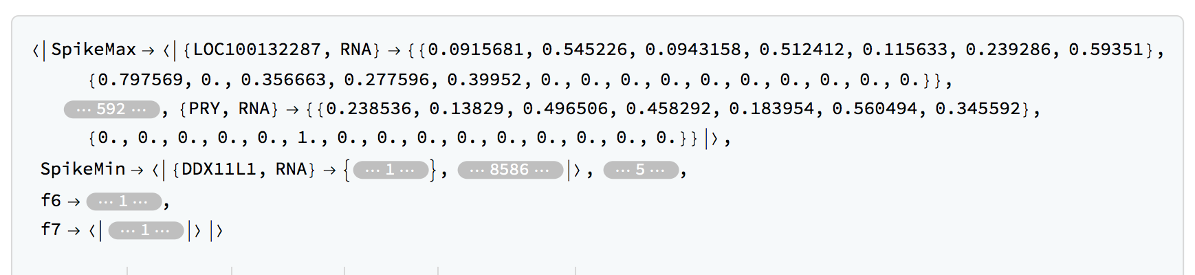
rnaClassification = TimeSeriesClassification[rnaFinalTimeSeries,timesRNA,LombScargleCutoff -> q95RNA,SpikeCutoffs -> q95RNASpikes]

We can get the number of members in each category:

Query[All, Length]@rnaClassification
(*<|"SpikeMax" -> 598, "SpikeMin" -> 8672, "f1" -> 62, "f2" -> 3, 
 "f3" -> 14, "f4" -> 42, "f5" -> 14, "f6" -> 10, "f7" -> 57|>, This will depend on the precise cutoffs used.*)

Also we can see what the frequencies are by simply running the LombScargle function over the desired times for one of the time series and set the FrequenciesOnly option:

LombScargle[rnaFinalTimeSeries[[1]], timesRNA, 
 FrequenciesOnly -> True]
(*<|"f1" -> 0.00500668, "f2" -> 0.0104306, "f3" -> 0.0158545, 
 "f4" -> 0.0212784, "f5" -> 0.0267023, "f6" -> 0.0321262, 
 "f7" -> 0.0375501|>*)

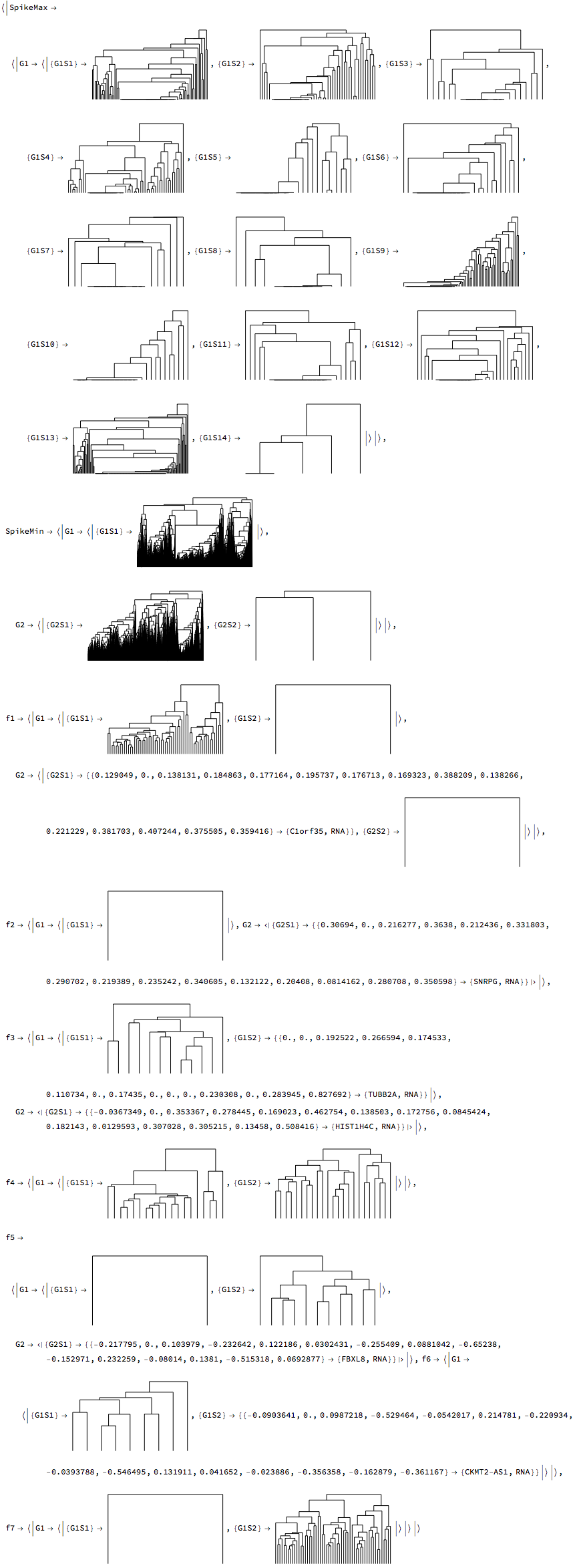
We now cluster our RNA data. A two-tier hierarchical clustering of the data is performed, using a set of two classification vectors, $\{\{\text{classification vector}_1\},\{\text{classification vector}_2\}\}$ for each time series to cluster the data pairwise. The vectors are typically the output from TimeSeriesClassification. Similarities at each clustering tier are then computed using in succession from each time series first $\{\text{classification vector}_1\}$, and subsequently $\{\text{classification vector}_2\}$ (which corresponds to the $\{\text{input data time series}\}$. The main idea is that signals can have similarity based on the periodogram - which will not be able to detect phase differences, and subsequent clustering based on real values which should detect phase differences. The result is grouping of the data based on similarity, denoted as G#S#, where G denotes the group based on the first clustering, and S denotes the corresponding subgroup for that group. For example G2S3 denotes the 3rd subgroup of group 2.

rnaClusters = TimeSeriesClusters[rnaClassification, PrintDendrograms -> True]

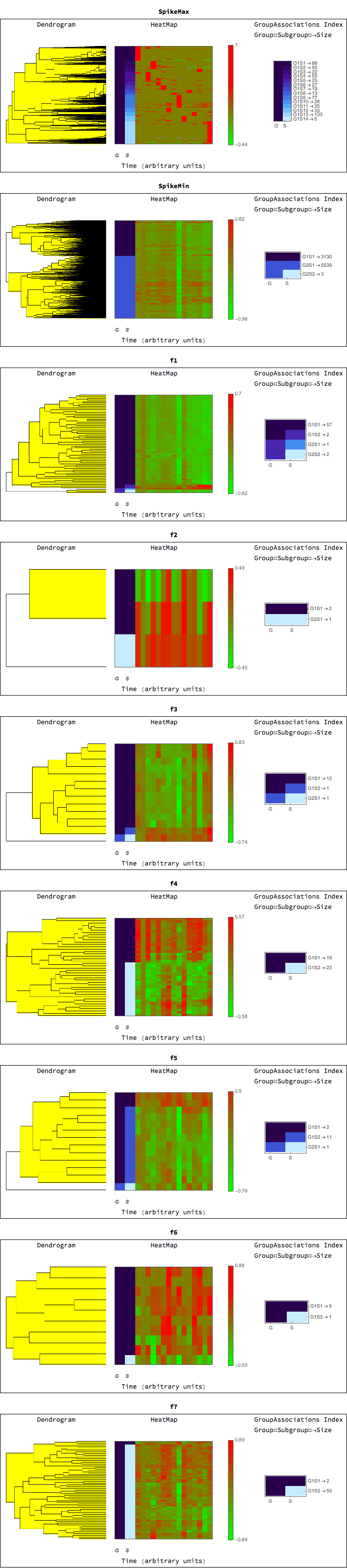
For each class we can generate a dendrogram/heatmap plot, with groupings represented on the left, and highlighted to represent the grouping level. The G, S, columns represent the groupings and subgroupings generated by the clustering. The legend shows the corresponding groupings and subgrouping, and the number of elements in each group subgroup.

TimeSeriesDendrogramsHeatmaps[rnaClusters]

Annotation Enumeration

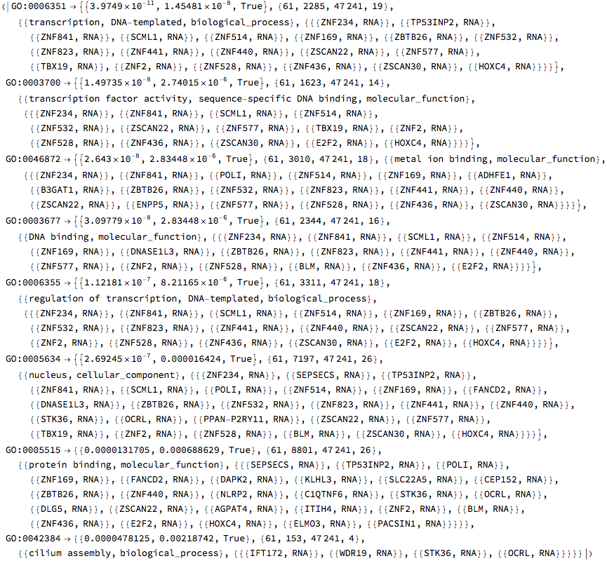
We can carry out Gene Ontology analysis using for all the classes and groups/subgroups. We only report terms for which there are at least 3 members (N.B. this may be a bit time consuming because of the number of tests running ~ few minutes). The output has enrichments for each class and group

goAnalysisRNA = GOAnalysis[rnaClusters, OntologyLengthFilter -> 3, ReportFilter -> 3 ]
Query[All, Keys]@goAnalysisRNA
(*<|"SpikeMax" -> {"G1S1", "G1S2", "G1S3", "G1S4", "G1S5", "G1S6", 
   "G1S7", "G1S8", "G1S9", "G1S10", "G1S11", "G1S12", "G1S13", 
   "G1S14"}, "SpikeMin" -> {"G1S1", "G2S1", "G2S2"}, 
 "f1" -> {"G1S1", "G1S2", "G2S1", "G2S2"}, "f2" -> {"G1S1", "G2S1"}, 
 "f3" -> {"G1S1", "G1S2", "G2S1"}, "f4" -> {"G1S1", "G1S2"}, 
 "f5" -> {"G1S1", "G1S2", "G2S1"}, "f6" -> {"G1S1", "G1S2"}, 
 "f7" -> {"G1S1", "G1S2"}|>*)

We can view results for any of the groups (and also check out the behavior using the heatmaps generated in the previous section

Query["SpikeMax", "G1S1"]@goAnalysisRNA

We can export the reports to excel spreadsheets, e.g.,

EnrichmentReportExport[goAnalysisRNA, OutputDirectory -> $UserDocumentsDirectory, AppendString -> "GOAnalysisRNA"];

We can also carry out KEGG: Kyoto Encyclopedia of Genes and Genomes pathway analysis for all the classes and groups/subgroups. We only report terms for which there are at least 2 members. Please note again that this is a time consuming computation for a large set (few minutes).

keggAnalysisRNA = KEGGAnalysis[rnaClusters, ReportFilter -> 2];

We can then view results for any of the groups (and also check out the behavior using the heatmaps generated in the previous section), e.g.:

Query["SpikeMax", "G1S2"]@keggAnalysisRNA

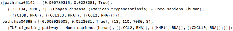
Let us look at the genes in our data belonging to one of these pathways:

pathwaymembers = 
 Query["SpikeMax", "G1S2", 2, 3, 2, All, 1]@keggAnalysisRNA
(*{{"CCL2", "RNA"}, {"MMP14", "RNA"}, {"CXCL10", "RNA"}} *)

We can obtain a link to the KEGG pathway of interest:

KEGGPathwayVisual["path:hsa04668"]
(*<|"Pathway" -> "path:hsa04668", "Results" -> {"http://www.kegg.jp/kegg-bin/show_pathway?map=hsa04668"}|>*)

And we can highlight the genes in the results in the pathway if we want (open the link in a browser to visualize):

KEGGPathwayVisual["path:hsa04668", MemberSet -> pathwaymembers]
(*<|"Pathway" -> "path:hsa04668","Results" -> {"http://www.kegg.jp/kegg-bin/show_pathway?map=hsa04668&multi_query=hsa%3A6347+%2380b2ff%2C%23000000%0D%0Ahsa%3A4323+%2380b2ff%2C%23000000%0D%0Ahsa%3A3627+%2380b2ff%2C%23000000%0D%0A"}|>*)

The figure can also be downloaded directly (not shown here due to copyright - please check if this is appropriate based on nature of your institution -academic vs. not with KEGG directly or read license distributed with MathIOmica):

KEGGPathwayVisual["path:hsa04668", ResultsFormat -> "Figure", 
 MemberSet -> pathwaymembers]