Message Boards Message Boards

Make a KAM Torus in Wolfram Language?

Posted 7 years ago

Hello everyone, I want to ask your help with the following problem I want to do the graph of the Kam Theorem, I started searching the internet about it, and I found the following link FRACTINT Kam Torus but I am not able to program it in Mathematica, then look for some example that was programmed in another language to have some clue how to do it and I saw the link that I then share Maple V and Fractals: KAM Torus, what happens is that I do not know anything about Maple software even though it seems a little to Mathematica, I do not understand much of the code presented in the above mentioned page, I would like that if someone understands the code in question please give me some tips to do the same in Mathematica. Thanks in advance (^_^)

POSTED BY: Luis Ledesma
9 Replies
Posted 7 years ago

Thanks for sharing the information, it's just amazing (-.-)

POSTED BY: Luis Ledesma

These pictures are really great, but I think Arnol'd ( the A of KAM ) would shake his head, reading this thread. Especially because these pictures aren't tori, but maybe they are Poincare sections. I don't know.

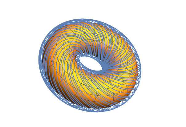
A KAM tori is really easy to make in any programming language. Start with a unit area that maps to the surface of a torus, and identify each dimension with a phase space angle of uncoupled harmonic oscillators. Third and fourth phase space dimensions can be constant conserved energies or one conserved energy and one conserved angular momentum. Time evolution has constant angular velocity in both phase spaces, so the graph is just a line in the unit area. Adding in the topology you have a line that (probably) goes dense on the surface of a Torus (or in the unit area). With angular velocity ratio $\sqrt{2}$:

Torus = {r Cos[\[Phi]], r Sin[\[Phi]], .5 Sin[\[Theta]]} /. {r -> (1 - 0.5 Cos[\[Theta]])};
Trajectory = {r Cos[\[Phi]], r Sin[\[Phi]], .6 Sin[\[Theta]]
} /. {r -> (1 - 0.6 Cos[\[Theta]])} /. {\[Theta] -> Sqrt[2] \[Phi]};
Show[
 ParametricPlot3D[Trajectory, {\[Phi], 0, 100 Pi}],
 ParametricPlot3D[Torus, {\[Phi], 0, 2 Pi}, {\[Theta], 0, 2 Pi}],
 Boxed -> False,
 Axes -> False
 ]
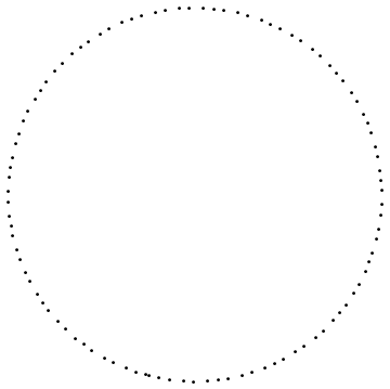
Graphics[Point@Trajectory[[1 ;; 2]] /. \[Theta] -> # 2 Pi & /@  Range[100]]

Wrapped Torus Poincare Section

  1. You can add a small r^4 perturbation, but then you need to change parameterization slightly. The advantage of r^4 is that angular momentum and energy are still constants. Using r^4 perturbation, it's possible to see precession, which is the one remarkable difference from the multi-periodic, harmonic example.

  2. If you add a perturbation with D4 symmetry, you lose conservation of momentum, but still have a three dimensional conserved energy surface, where I think it's possible for chaos to happen. Then you will get some pictures like the above by taking Poincare sections, and it will be more intelligible and less plagiarism. Note: I do not recommend triangular Henon Heiles, as odd powers potentials are more difficult to work with than strictly even.

So my suggestion is basically don't jump to stage 3 or 4 before you go through the basics. Ignore this advice at the risk of delusion, confusion, etc.

If you have never done phase space geometry before, my article Plane Pendulum and Beyond is a beginner introduction, where you can pick up some of the basic ideas of symplectic geometry without needing to worry about what Darboux's theorem looks like on a banquet table, and does it apply to dessert?

Best Regards.

POSTED BY: Brad Klee
Posted 7 years ago

Michael Helmle, thank you very much for your help, I think your compiled version is interesting, since you are using mathematica functions, I am learning more from the users of this community, thanks again.

Postscript, I'm reviewing your code step by step to understand it better. (^_^)

POSTED BY: Luis Ledesma
Posted 7 years ago

I found another issue with the compiled function implementation: i had already assigned a numerical value to "angle" in my notebook and was not aware of it, but when you do a clean restart and this is not the case then the compiled function will not build correctly. In consequence the angle variable has also to be put in the interface to the compiled function. So below is a corrected version and I checked it with a clean restart.

f1 = Compile[{{xy, _Real, 1}}, 
   Module[{cs = Cos[xy[[3]]], sn = Sin[xy[[3]]], x = xy[[1]], 
     y = xy[[2]]}, {N[x cs + (x^2 - y) sn], 
     N[x sn - (x^2 - y) cs], xy[[3]]}]];

kamtorus2[ angle_, step_, ende_, points_] := 
 Module[{ x, xold, y, orbit},
  For[orbit = 0, orbit < ende, orbit += step,
   pts = AppendTo[pts, 
      NestWhileList[f1, {orbit/3., orbit/3., angle}, 
       Total[Abs[#]] < 2. 10^38 &, 1, points ]];
   ]]

pts = {};
Timing[kamtorus2[1.3, 0.05, 1.5, 200]]
ListPlot[Flatten[pts, 1][[All, 1 ;; 2]], AspectRatio -> 1]

Now it should compile and run smoothly and the output reacts to the setting of angle

POSTED BY: Michael Helmle
Posted 7 years ago

Sorry, forgot to copy the compiled function f1: Here is a more Mathematica style implementation (which runs faster):

f1 = Compile[{{xy, _Real, 1}}, 
  Module[{cs = Cos[angle], sn = Sin[angle], x = xy[[1]], 
    y = xy[[2]]}, {N[x cs + (x^2 - y) sn], 
    N[x sn - (x^2 - y) cs]}]]

kamtorus2[ angle_, step_, ende_, points_] := 
 Module[{ x, xold, y, orbit},
  For[orbit = 0, orbit < ende, orbit += step,
   pts = AppendTo[pts, 
      NestWhileList[f1, orbit/3. {1, 1}, Total[Abs[#]] < 2. 10^38 &, 
       1, points ]];
   ]]

pts = {};
Timing[kamtorus2[1.3, 0.05, 1.5, 200]]
ListPlot[Flatten[pts, 1], AspectRatio -> 1]
POSTED BY: Michael Helmle
Posted 7 years ago

Here is a more Mathematica style implementation (which runs faster):

kamtorus2[ angle_, step_, ende_, points_] := 
 Module[{ x, xold, y, orbit},
  For[orbit = 0, orbit < ende, orbit += step,
   pts = AppendTo[pts, 
      NestWhileList[f1, orbit/3. {1, 1}, Total[Abs[#]] < 2. 10^38 &, 
       1, points ]];
   ]]

pts = {};
Timing[kamtorus2[1.3, 0.05, 1.5, 200]]
ListPlot[Flatten[pts, 1], AspectRatio -> 1]
POSTED BY: Michael Helmle

Beautiful code, @Michael Helmle, but is f1 defined? Last code is not producing proper image.

POSTED BY: Sam Carrettie
Posted 7 years ago

Below is a somewhat naive implementation.

kamtorus[ angle_, step_, ende_, points_] := 
 Module[{ x, xold, y, orbit},
  For[orbit = 0, orbit < ende, orbit += step,
   x = orbit/3.;
   y = x;
   ptno = 0;
   While[Abs[x] < 1. 10^38 && Abs[y] < 1. 10^38 &&  ptno < points,
    xold = x;
    x = N[ x        Cos[angle] +     (x^2 - y) Sin[angle]];
    y =  N[ xold Sin[angle] - (xold^2 - y) Cos[angle]];
    pts = AppendTo[pts, {x, y}];
    ptno++
    ];
   ]
  ]

pts = {};
Timing[kamtorus[1.3, 0.05, 1.5, 200]]
ListPlot[pts, AspectRatio -> 1]

enter image description here

POSTED BY: Michael Helmle
Reply to this discussion
Community posts can be styled and formatted using the Markdown syntax.
Reply Preview
Attachments
Remove
or Discard

Group Abstract Group Abstract