GOAL OF THE PROJECT
During Wolfram Summer School 2017, I set out to create an efficient quantum computing framework in Mathematica. Prior to this project, there were already several quantum computing packages for Mathematica, including Quantum, QuCalc, and Quantum Computing with the Wolfram Language, the last of which was a product of WSS 2016. However, there was no existing package that was hassle-free, and provided a unified representation of the various types of quantum systems one might want to use in computations. I set out to allow users to simulate quantum circuit computations on all of these types of quantum states - which I will go into shortly.
My main goal, however, was to make the circuit computations as fast - and scalable - as possible. The main difficulty that arises when simulating quantum systems on classical computers is that a quantum system with $~{O}(n)~$ quantum bits, or qubits, requires a representation consisting of $~O(2^n)~$ classical bits. From the start, I knew that my primary task would consist of designing an architecture for the framework that would facilitate these computations.
Background
Before I get into the specifics of my implementation, I'm going to review some of the basics of quantum computing:
Quantum States
In classical computing, information is stored in bits, i.e. $~0~$'s and $~1~$'s. At any point in time, each bit is in one of these two states. Operations such as "AND", "NOT", and "Controlled-NOT" gates take bits as input, and output other bits.
In quantum computing on the other hand, the fundamental unit is the qubit, or quantum bit. A qubit lives in a Hilbert space $~H = \mathbb{C}^2~$. Rather than take values in $\{0,1\}$, a qubit can take any complex-valued state $\begin{bmatrix} \alpha \\ \beta \end{bmatrix}$ that is normalized: $\|\alpha \|^2+ \|\beta \|^2 = 1$.
Rewriting this as $\alpha \begin{bmatrix} 1 \\ 0 \end{bmatrix} + \beta \begin{bmatrix} 0 \\ 1 \end{bmatrix} $, we can view the qubit as a linear combination, or superposition of the two basis states $ \begin{bmatrix} 1 \\ 0 \end{bmatrix} $ and $ \begin{bmatrix} 0 \\ 1 \end{bmatrix} $, and subsequently treat these as our quantum analogs of $0$ and $1$ so that we can perform quantum computations.
During computation, a qubit does not have to take on either of its basis states. Rather, it "collapses" into one of its eigenstates when it is measured at the end of a computation. A computation consists of any unitary operator acting on the state of the qubit.
Things get more interesting when we consider a composite quantum state, made up of multiple qubits. A quantum state comprised of two qubits, $q_a$ and $q_b$, lives in $~ \mathbb{C}^4~$. In the computational basis, $ \begin{bmatrix} 1 \\ 0 \\ 0 \\ 0 \end{bmatrix} $ describes the state in which $q_a$ and $q_b$ are both 0, $ \begin{bmatrix} 0 \\ 1 \\ 0 \\ 0 \end{bmatrix} $ corresponds to $0$ for $q_a$ and $1$ for $q_b$, $ \begin{bmatrix} 0 \\ 0 \\ 1 \\ 0 \end{bmatrix} $ to $1$ for $q_a$ and $0$ for $q_b$, and $q_b$, $ \begin{bmatrix} 0 \\ 0 \\ 0 \\ 1 \end{bmatrix} $ to $1$ for both qubits.
Unlike in the classical case, in quantum physics it is often not possible to decompose the state of a composite system into separate states for each subsystem. For example, no matter the choice of $\alpha$, $\beta$, $\gamma$ and $\delta$, it is not possible to write $ \frac{1}{\sqrt{2}}\begin{bmatrix} 1 \\ 0 \\ 0 \\ 1 \end{bmatrix} = \begin{bmatrix} \alpha \\ \beta \end{bmatrix} \otimes \begin{bmatrix} \gamma \\ \delta \end{bmatrix}$. In such a scenario, the state is said to be entangled.
We can make things even MORE interesting by adding in statistical uncertainty. So far, we have been discussing what are referred to as pure states. Even though we have allowed qubits to be in superposition states, we were always sure to be in that superposition. A mixed state is a statistical ensemble of pure states. For example, $q_a$ could have a $50\%$ chance of being in the state $\begin{bmatrix} 0 \\ 1 \end{bmatrix}$ and a $50\%$ chance of being in the state $\frac{1}{\sqrt{2}} \begin{bmatrix} 1 \\ 1 \end{bmatrix}$.
Okay, just one more complication: remember how we began by drawing the analogy between bits and qubits? We can extend this analogy to general digit systems. A classical system that can be in one of the d states $\{0, 1, \dots, d-1\}$ is transformed into a qudit: a normalized complex-valued state in $~ \mathbb{C}^d~$, which takes on superpositions of its $d$ basis states.
My framework treats pure unentangled and entangled states, mixed states, qubits and qudits on the same footing.
Quantum Circuits
As I mentioned above, a computation consists of any unitary operator acting on your quantum state. If you are performing computations on many qudits, as is often necessary for the design of complex circuits, these operations essentially become large matrix multiplications. For example, an operation performed on 4 qutrits (three level quantum systems), would involve multiplying your state vector by a matrix of size $3^4 \times 3^4$. One can imagine how quickly this scaling becomes a performance issue.
Design
In my framework, the basic data structures are QuantumObservable and QuantumState. A QuantumObservable consists of a Hermitian matrix and a description. A QuantumState consists of a density matrix, represented as a sparse array, a lookup table that associates row and column indices with combined computational basis states of the system, and an ordered list of quantum objects that comprise the state. For example,
psi = CreateQuantumState["w2" -> {0.4, 0.8}, {"w1", "w3"} -> {{0, .1, .9}, {.2, .4, .3}}]
returns a QuantumState consisting of quantum objects "w1", "w2", and "w3". 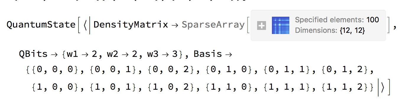 .
.
"w1" and "w2" are qubits, while "w3" is a qutrit. "w1" and "w3" are input as one 2-dimensional array because they are entangled, and cannot be represented independently. The state is automatically normalized.
We can visualize the density matrix of the state using QuantumPlot[psi].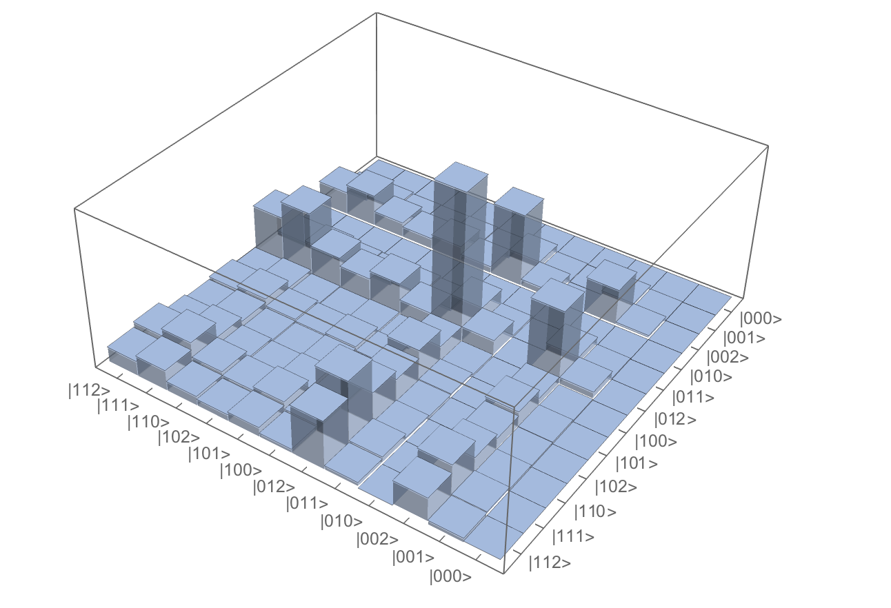
We can query the state to see whether it is pure, mixed, or entangled (for pure states) with commands like EntangledQuantumStateQ.
Note that we represent all states in terms of density matrices rather than state vectors so that the architecture is consistent for pure and mixed states. This does not impact performance because we are using sparse arrays.
Quantum Operations
In my framework, quantum operations are not hard-coded as matrices. Instead, they are defined by rules which, for a d-dimensional quantum state, will apply the d-dimensional version of the operation. In order to avoid matrix multiplications, two-qudit operations like "CNOT" and "SWAP" are implemented through array reshaping and manipulation rather than being explicitly constructed.
Quantum Circuit
One of the most important aspects of my project is quantum compilation. A quantum circuit can be created either by giving a list of quantum operations, or concatenating other circuits. The quantum circuit is left unevaluated until it acts on a quantum state, at which time it is simplified by a host of pattern-based algebraic identities. This compilation reduces the number of operations in the circuit, minimizing the number of full-blown matrix multiplications.
Other Features
I also implemented a function to get the Von Neumann entropy of a quantum state, a partial trace function to produce the quantum state formed by tracing out subsystems, and a measurement function which calculates the expectation value of an observable on any quantum state.
SUMMARY OF WORK
This Quantum Computing framework enables the simulation of quantum circuits for qudits (generalized d-level quantum systems. Using sparse arrays and lookup tables, this package efficiently stores quantum states, maintaining a unified structure for pure, mixed, and entangled quantum states. The user can create an initial quantum state, and generate a quantum circuit - either out of individual gate operations or by concatenating other circuits. The crux of the framework is quantum circuit compilation: The circuit is not evaluated until it acts on an input quantum state, and using pattern matching I implement a variety of algebraic simplification rules to minimize the number of matrix multiplications.
Future Work
Obviously, there are a plethora of quantum computing features I would have liked to implement had I had more time. In the future, I hope to add functionality for combining quantum states, as well as incorporating a wider variety of multi-qudit operations. In addition, I would like to include functions for well-known quantum algorithms such as Deutsch's, Grover's, and Shor's algorithms so that the user can apply them directly to a quantum state.


