Introduction
The problem to solve is easy to state: What does the following image say? 
At first, this may seem as a trivial problem, but sometimes it is not straigthforward for us to understand someone else's handwriting. How difficult is it for a Neural Network to understand handwritten words or sentences? The goal of this project was to build a Neural Network that could identify and return individual characters that appear in images of handwritten words or sentences.
Collecting the data
The first step was to collect available data. The IAM Handwriting Database 3.0 was this project's source for images of handwritten text. The database is available in different formats and is structured as follows:
- Handwriting samples of 657 writers:
- 1539 pages of scanned text
- 5685 sentences
- 13353 lines
- 115320 words
For this project, only the lines and words sets were used.
Wrangling the labels
Labels were obtained via the IAM Database webpage (sign in required):
data = Import["http://www.fki.inf.unibe.ch/DBs/iamDB/data/ascii/words.txt"] // StringDrop[#, 802] &
The text file was imported as a string and had to be edited because of many inconsistencies in the data. In the case of words, this was done to edit the string in an appropriate way for our purposes:
dataTidy =
 StringReplace[data, "n log n" -> "nlogn"] //
       StringReplace[#, "B B C" -> "BBC"] & //
      StringReplace[#, "M P" -> "MP"] & //
     StringReplace[#, "A T V" -> "ATV"] & //
    StringReplace[#, "I T V" -> "ITV"] & //
   StringReplace[#, x : "NN " ~~ "T V" :> x <> "TV"] & //
  StringReplace[#, "T C O" :> "T CO"] &
The stringwas partitioned according to the number of columns in the dataset:
dataList = (StringSplit[dataTidy] // Partition[#, 9] & )
These are the column names:
colNames =
 StringSplit@
  "word_id segmentation_result graylevel x_bounding y_bounding w_bounding h_bounding gramm_tag transcription"
We create an association between the column names and the actual data, then we transform it into a dataset:
dataSet =
  Association @@@
    Table[colNames[[i]] -> (dataList)[[j, i]], {j, 1,
      Length[dataList]}, {i, 1, Length[colNames]}] // Dataset;
The image data is too large to import it, so we will have to do out-of-core training. We need to obtain the filenames:
fileNames = FileNames["*.png", FileNameJoin[{NotebookDirectory[], "words"}], Infinity]
Now we need to create the directories in which the preprocessed images will be:
newDirectories =
  StringReplace[#,
       "\\" ~~ LetterCharacter ~~ DigitCharacter .. ~~ "-" ~~
         DigitCharacter .. ~~ LetterCharacter | "" ~~ "-" ~~
         DigitCharacter .. ~~ "-" ~~ DigitCharacter .. ~~ ".png" ->
        ""] & /@ fileNames //
    StringReplace[#, "words" -> "words_resized"] & //
   DeleteDuplicates;
CreateDirectory[File@#] & /@ newDirectories;
Now we create the filenames of the new images:
exportFileNames =
 StringReplace[#, "words" -> "words_resized"] & /@ fileNames
Wrangling the images
The varying dimensionality of the data was the first problem encountered. As it can be seen in the two plots below, there were very small images, mostly of punctuation marks, in the word set, whereas, compared to the others, many images were very large in the sentence set.
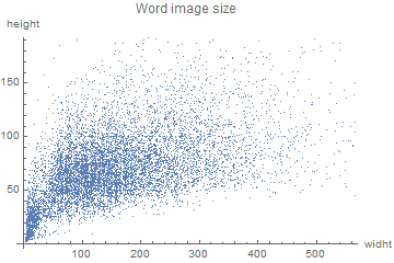
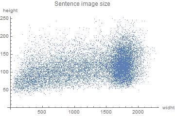
One of the models could handle images with one varying dimension, whereas the other models could only handle images of the same size. This, combined with the use of two different sets of data, led to the preprocessing of the images in many different ways:
Sentences:
- Grayscaled images with varying length, but with a heigth of 161.
- Binarized images with varying length, but with a heigth of 161.
- Images reshaped to {1100, 90}.
Words:
- Images were reshaped to have either a width of 128 or a height of 32, then they were centered and overlaid on a white background. The resulting image was of size {128,32}.
- Images were reshaped to have either a width of 128 or a height of 32, then they were overlaid and positioned to the left of a white background. The resulting image was also of size {128,32}.
Sentences preprocessing
Sentences in point 1 were reshaped and stored in the hard drive in the following way:
ParallelMap[
 Export[exportFileNames[[#]],
   ImageResize[Import[fileNames[[#]]], {161, Automatic}]] &,
 Range[Length[fileNames]]
]
Sentences in point 2 were reshaped, binarized and stored in the hard drive in the following way:
ParallelMap[
 Export[exportFileNames[[#]],
   ImageResize[Binarize@Import[fileNames[[#]]], {161, Automatic}]] &,
 Range[Length[fileNames]]
]
Sentences in point 3 were reshaped using the function NetEncoder in the following manner:
encoder = NetEncoder[{"Image", {1100}, "ColorSpace"-> "Grayscale"}]
Words preprocessing
In order to preprocess words in a more appropriate way, some functions had to be defined. The arguments for the function reshape are the image, the width and height targets.
reshape = Function[{image0, widthTarget0, heigthTarget0} ,
   Module[{image = image0, widthTarget = widthTarget0,
     heigthTarget = heigthTarget0, width, heigth , fx, fy, f,
     newSize, resizedImage},
    {width, heigth} = ImageDimensions[image];
    fx = width/widthTarget;
    fy = heigth/heigthTarget;
    f = Max[fx, fy];
    newSize = {Max[Min[widthTarget, Round[width/f]], 1],
      Max[Min[heigthTarget, Round[heigth/f]], 1]} ;
    resizedImage = ImageResize[image, newSize];
    resizedImage
    ]];
The function imageInRectangle, as it name implies, overlays the word image on a white background of size {128,32}.
imageInRectangle = Function[{image0, widthTarget0, heigthTarget0} ,
   Module[{image = image0, rectangle , widthTarget = widthTarget0, heigthTarget = heigthTarget0, composedImage},
    rectangle = Rasterize[Graphics[{White, Rectangle[]}], ImageSize -> {128, 32}];
    composedImage =
     ImageCompose[rectangle, reshape[image, widthTarget, heigthTarget], {Center}];
    composedImage
    ]];
Word images were exported in a similar fashion to what was done in the Sentences preprocessing subsection.
Neural Networks
Relevant data
Only the relevant data for our purposes was kept:
modifiedLabels = imageAndLabels[[1 ;;, 2]]  // Normal;
modifiedImages = File[#] & /@ exportFileNames5;
modifiedData =
 Table[modifiedImages[[n]] ->  modifiedLabels[[n]], {n, 1,
   Length[modifiedImages], 1}]
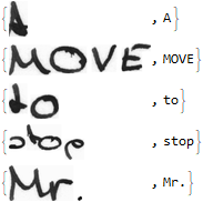
Resulting in the following structure:
The data was divided into a train and a test set:
{testData, trainData} =
  TakeDrop[modifiedData , Ceiling[Length[dataSet]/10]];
Connectionist Temporal Classification
Connectionist Temporal Classification is both a type of neural network output and a loss function. It is useful for training Recurrent Neural Networks (RNN) in which the input is sequential, like handwriting recognition. In our case, the inputs were images of handwritten words or sentences, and the output was a sequence of characters. To simplify the problem, only lower case characters were considered in the data.
The following decoder was used:
chars = Keys@
  KeySort@Counts@Flatten@Characters@modifiedData [[1 ;;, 2]]
decoder = NetDecoder[{"CTCBeamSearch", chars, "BeamSize" -> 50}]
The following loss function was used:
ctcLoss = CTCLossLayer["Target" -> NetEncoder[{"Characters", chars}]]
The encoder varied depending on the input data, but one of the word image encoders was the following one:
encoder = NetEncoder[{"Image",{128,32}, "ColorSpace"-> "Grayscale"}]
The model with the lowest loss was the following one (this one used all available characters):
convNet = NetInitialize@NetChain[{ConvolutionLayer[32, 5],
    BatchNormalizationLayer[],
    Ramp,
    PoolingLayer[2],
    ConvolutionLayer[64, 5],
    BatchNormalizationLayer[],
    Ramp,
    PoolingLayer[2],
    ConvolutionLayer[128, 3],
    BatchNormalizationLayer[],
    Ramp,
    PoolingLayer[2],
    ConvolutionLayer[128, 3],
    BatchNormalizationLayer[],
    Ramp,
    PoolingLayer[2],
    ConvolutionLayer[256, 3],
    BatchNormalizationLayer[],
    Ramp,
    PoolingLayer[2],
    FlattenLayer[1],
    TransposeLayer[],
    GatedRecurrentLayer[256],
    GatedRecurrentLayer[256],
    NetMapOperator[LinearLayer[Length[chars] + 1]],
    SoftmaxLayer[]
    },

   "Input" -> encoder,
   "Output" -> decoder]
Training the model:
convNetTrain =
 NetTrain[convNet, trainData, LossFunction -> ctcLoss,
  MaxTrainingRounds -> 20, ValidationSet -> testData,
  TargetDevice -> "GPU", BatchSize -> 32]
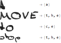
Unfortunately, this model was not good enough, since the loss reached only 1.92 during training. This might probably be because of vanishing gradient problems. Even though some corrections were made to solve this problem, the previous model still obtained a better loss than the rest.
These are the outputs it gives when feeded an image:
Conclusions
Despite several attempts, the results obtained using Convolutional and Recurrent Neural Networks were not satisfying. The main reason behhind this underperformance might be vanishing gradient problems.
Further explorations
- Curate a better dataset.
- Implement other kinds of networks to this problem (Densenet).
Script
To train the neural network, please follow this link and download the script (image data should already be in a directory named "~/words"):


