Open in Cloud | Download to Desktop via Attachments Below
Briefly, a continued logarithm is an arbitrarily long bit string approximating a real number arbitrarily well, and supports arbitrarily precise bit-at-a-time algorithms for rational functions of these numbers. (See http://www.tweedledum.com/rwg/cfup.htm , p 47+)
A six-bits-per-term $\pi$ series:
Product[MatrixForm@{{512 k^3, 0}, {32 k^3 (-37 + 42 k), (-1 + 2 k)^3}}, {k, ?}] ==
 MatrixForm[{{oo ?, 0}, {oo, "?"}}]
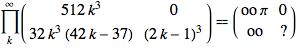
Where ? means matrix product, not Mathematica product, and oo is some quantity that blows up with the number of product terms, the same way you compute continued fractions with 2*2 matrices. An incorrect form of this series is derived in https://dspace.mit.edu/handle/1721.1/6088 . We initialize the work matrix m to the first term of the matrix product:
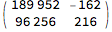
MatrixForm[ m = {{512 k^3, 0}, {32 k^3 (-37 + 42 k), (-1 + 2 k)^3}} /. k -> 1]

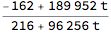
This represents the function
Divide @@ (m.{t, 1})

where t is the tail of the series, starting with k=2 rather than 1. It should be easy to show that, in general,
3/8/k < t < 3/8/(k + 1)
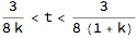
giving bounds
m /. {{t -> 3/8/1.}, {t -> 3/8/2.}}
{3.14754, 3.09677}
Since these both exceed 2, we commence output with
Style[cl@? = {1}, 22]

and left multiply m by the divide-by-2 matrix:
MatrixForm[m = {{1, 0}, {0, 2}}.m]

It costs almost nothing to remove the common power of 2:
MatrixForm[m = m/2]

representing the function
Divide @@ (m.{t, 1})

We still are on input term k=1, and can still use
% /. {{t -> 3/8/1.}, {t -> 3/8/2.}}
{1.57377, 1.54839}
which is smack between 1 and 2, which we celebrate with
Style[AppendTo[cl@?, 0], 22]

and left multiply m by the subtract-1-and-reciprocate matrix:
(m = {{0, 1}, {1, -1}}.m) // MatrixForm

representing
Divide @@ (m.{t, 1})

Again using
% /. {{t -> 3/8/1.}, {t -> 3/8/2.}}
{1.74286, 1.82353}
which dictates another
Style[AppendTo[cl@?, 0], 22]
and
(m = {{0, 1}, {1, -1}}.m) // MatrixForm

representing
Divide @@ (m.{t, 1})

% /. {{t -> 3/8/1.}, {t -> 3/8/2.}}
{1.34615, 1.21429}
Style[AppendTo[cl@?, 0], 22]
(m = {{0, 1}, {1, -1}}.m) // MatrixForm

Divide @@ (m.{t, 1})

% /. {{t -> 3/8/1.}, {t -> 3/8/2.}}
{2.88889, 4.66667}
This unambiguously exceeds 2, so
Style[AppendTo[cl@?, 1], 22]
MatrixForm[m = {{1, 0}, {0, 2}}.m]

Divide @@ (m.{t, 1})

% /. {{t -> 3/8/1.}, {t -> 3/8/2.}}
{1.44444, 2.33333}
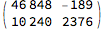
Our interval of uncertainty contains 2! At last we gobble (right multiply) the k=2 term.
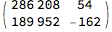
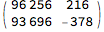
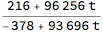
MatrixForm[ m = m.{{512 k^3, 0}, {32 k^3 (-37 + 42 k), (-1 + 2 k)^3}} /. k -> 2]
Divide @@ (m.{t, 1})
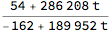
(Remembering to bump k !)
% /. {{t -> 3/8/2.}, {t -> 3/8/3.}}
{1.51515, 1.51938}
(Giving six more bits of precision!)
Style[AppendTo[cl@?, 0], 22]
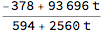
(m = {{0, 1}, {1, -1}}.m) // MatrixForm
Divide @@ (m.{t, 1})
% /. {{t -> 3/8/2.}, {t -> 3/8/3.}}
{1.9412, 1.92538}
Style[AppendTo[cl@?, 0], 22]
(m = {{0, 1}, {1, -1}}.m) // MatrixForm
Divide @@ (m.{t, 1})
% /. {{t -> 3/8/2.}, {t -> 3/8/3.}}
{1.06248, 1.08064}
Style[AppendTo[cl@?, 0], 22]
(m = {{0, 1}, {1, -1}}.m) // MatrixForm

Divide @@ (m.{t, 1})
% /. {{t -> 3/8/2.}, {t -> 3/8/3.}}
{16.0056, 12.4004}
Whoa, a burst of three 1s!
Style[AppendTo[cl@?, 1]; AppendTo[cl@?, 1]; AppendTo[cl@?, 1], 22]

MatrixForm[m = {{1, 0}, {0, 8}}.m]
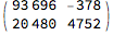
MatrixForm[m = m/2]
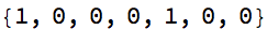
(Since we knew it was three ones and not four, we could have output 1,1,1,0 and left multiplied m by
MatrixForm[{{0, 1}, {1, -1}}.{{1, 0}, {0, 8}}]

This process may be continued indefinitely, or until the integers in m overflow.
 Attachments:


