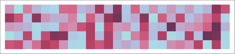
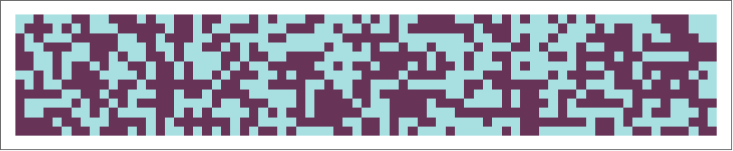
 A visualization of random reals
  A visualization of rule 30
Introduction
This project aims to implement systematic randomness testing into the Wolfram Language through both theoreticallydesigned tests and Monte Carlodesigned tests. The tests use a sequence of either zeros and ones or reals between zero and one as input. The tests return a pvalue evaluating the null hypothesis that the sequence is indeed random. The general design of the tests is to first create a test statistic based on some property of random sequences. A sampling distribution is then derived either theoretically or using a Monte Carlo method in order to generate the pvalues.
The project implements equidistribution and diehard tests in order to evaluate the randomness of a sequence. The general applications of a the project include evaluating random number generation techniques like linear feedback shift registers or cellular automata rules or evaluating the quality of a statistical sampling technique.
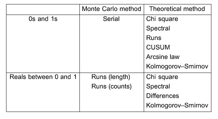
The following is a list of tests that are developed by method and type:
List of resource functions:
Using tests abbreviated documentation:
ResourceFunction["TestName"][sequence]
Returns a pvalue associated with sequence
ResourceFunction["TestName"][sequence,"TestStatistic"]
Returns the test statistic associated with sequence
ResourceFunction["TestName"][sequence,"PValue"]
Returns a pvalue associated with sequence
Implementing tests
Chi square equidistribution test
The first test we will examine is a relatively simple, ubiquitous test: the chi square test for independence. In this approach we will use the chi square test to measure how the observed values differ from expected values.
Zeros and ones
The expected value distribution of zeros and ones is very simple. There is a 1/2 probability that a variate will be 0 and a 1/2 probability that a variate will be 1. Therefore, we can set up a statistic like the following:
chiSquareTestStatIntegers[seq_] := (Total[seq] - 1/2 Length[seq])^2/(
   1/2 Length[
     seq])(*observed number of ones*)+ ((Length[seq] - Total[seq]) -
     1/2 Length[seq])^2/(1/2 Length[seq])(*observed number of zeros*);
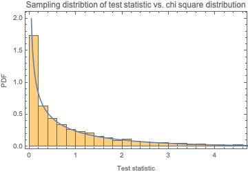
We know that this statistic will follow a chi square distribution with d.f. = 1. Let's confirm:
Show[Histogram[
  Table[chiSquareTestStatIntegers[RandomInteger[{0, 1}, 10000]],
   100000], Automatic, "PDF"],
 Plot[PDF[ChiSquareDistribution[1], x], {x, 0, 10},
  PlotRange -> {0, 2}], Sequence[
 PlotLabel -> "Sampling distribtion of test statistic vs. chi square \
distribution", Frame -> True, FrameLabel -> {"Test statistic", "PDF"}]
 ]
Therefore, we can construct a p-value as follows:
chiSquareTestPValueIntegers[seq_] :=
 1. - CDF[ChiSquareDistribution[1], chiSquareTestStatIntegers[seq]]
Random reals between zero and one
Again, with the chi square test for independence, we must compare observed values to expected values. For continuous distributions, we must choose bins in which we have expected values. For our purposes, we will choose bins of size 1/n where n is the length of the sequence. Using this bin specification, we know that the expected number of numbers we should observe in each bin should be 1. With this information, we can create a test statistic:
chiSquareTestStatReals[seq_] :=
 Total[(BinCounts[seq, 1/Length[seq]] - 1)^2/
  1](*note we use the listable atribute of squaring and basic \
arithmetic*)
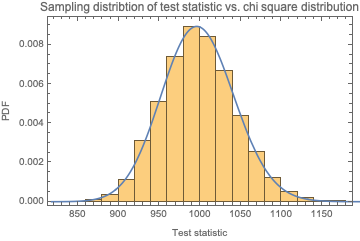
This distribution should follow the chi square distribution with d.f. = n -2 where n is the length of the sequence. Let's confirm:
Show[Histogram[
  Table[chiSquareTestStatReals[RandomReal[{0, 1}, 1000]], 10000],
  Automatic, "PDF"],
 Plot[PDF[ChiSquareDistribution[998], x], {x, 0, 1500},
  PlotRange -> {1.*^-6, All}], Sequence[
 PlotLabel -> "Sampling distribtion of test statistic vs. chi square \
distribution", Frame -> True, FrameLabel -> {"Test statistic", "PDF"}]
 ]
The KolmogorovSmirnov distribution fit test
The KolmogorovSmirnov test is a powerful distribution fit test that compares an empirical CDF to a defined CDF. The KolmogorovSmirnov test is relatively simple to formulate, but fortunately, it is already implemented in the Wolfram Language. We can then apply it to test for equidistribution of a sequence:
sequence = RandomReal[{0, 1}, 10000];
KolmogorovSmirnovTest[sequence, UniformDistribution[]]
This expression returns a pvalue.
Serial test
The serial test examines the frequency of the following pairs within the overall sequence:
{0, 0} {0, 1} {1, 0} {1, 1}
For example, the sequence
{1, 1, 0, 1, 0, 1, 1, 0, 0, 1, 1, 0, 1, 1, 1, 0, 1, 1, 1, 1, 0, 0,
   1, 0, 1, 1, 0, 0, 1, 0, 0, 1, 1, 0, 0, 1, 1, 0, 0, 0, 1, 1, 0, 1,
  1, 0, 0, 0, 0, 0, 1, 1, 1, 0, 1, 1, 1, 1, 1, 0, 0, 0, 0, 0, 1, 1, 0,
   0, 1, 1, 0, 0, 1, 1, 0, 0, 0, 0, 0, 1, 1, 1, 1, 0, 0, 1, 0, 1, 0,
  0, 0, 1, 1, 1, 1, 0, 1, 0, 1, 0}
has the associated counts
{16, 23, 24, 21}
where the order is that of the pairs list above. We can create a chi squarelike statistic that measures the deviation from expected frequency:

where n is the sequence length and µ_freq is the expected frequency with which the the pair occurs. These frequencies are computed empirically:
mcts[n_, samplesize_] :=
  Mean[Table[
    N@SequenceCount[RandomInteger[{0, 1}, n], #] & /@
     Tuples[{0, 1}, 2], samplesize]];
We can observe how these expected frequencies vary with sequence length:
{pts00, pts01, pts10, pts11} =
  ParallelTable[{{n, n, n, n}, mcts[n, 10000]/n}\[Transpose], {n, 500,
      10000, 500}]\[Transpose];
ListPlot[{pts00, pts01, pts10, pts11}, Frame -> True,
 FrameLabel -> {"Sequence length", "Mean pair counts ratio"}]
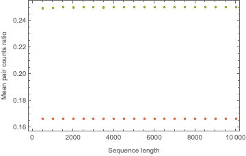
This figure displays how the expected frequencies are invariant under sequence length variation. After discovering this, we can come up with one set of constants that will work for any sequence length:
In[]:= $mctsrat = mcts[1000, 100000]/1000
Out[]:={0.166564, 0.249761, 0.249774, 0.166603}
And with this in mind we can finally construct a test statistic:
SerialTestStat[seq_] :=
  Total[((SequenceCount[seq, #] & /@ Tuples[{0, 1}, 2]) -
     Length[seq] $mctsrat)^2/(Length[seq] $mctsrat)];
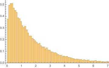
As we chose a chi squarelike statistic, we can anticipate that the test statistic will follow a gamma distribution.
serialsamplingdist[n_, samplesize_] :=
 ParallelTable[SerialTestStat[RandomInteger[{0, 1}, n]], samplesize]
serialdistsample1000 = serialsamplingdist[1000, 100000];
Histogram[serialdistsample1000, {.1}, "PDF"]
In[]:= serialfitdist1000 =
 FindDistribution[serialdistsample1000,
  TargetFunctions -> {GammaDistribution}]
Out[]:= GammaDistribution[1.12212, 1.53172]
.
Show[Histogram[serialdistsample1000, {.1}, "PDF"],
 Plot[PDF[serialfitdist1000, x], {x, 0, 10}]]
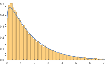
We can see that this distribution fits relatively well. Let's now investigate how the distribution parameters alpha and beta vary with sequence length.
\[Alpha]\[Beta]params[n_, samplesize_] :=
 FindDistributionParameters[serialsamplingdist[n, samplesize],
  GammaDistribution[\[Alpha], \[Beta]]]
paramvslength =
 Table[{{n,
      n}, {\[Alpha], \[Beta]}}\[Transpose] /. \[Alpha]\[Beta]params[n,
     10000], {n, 100, 10000, 1000}]
Row@{ListPlot[paramvslength\[Transpose][[1]], Sequence[
   ImageSize -> Medium, PlotLabel -> "\[Alpha]",
    PlotRange -> {0, All}]],
  ListPlot[paramvslength\[Transpose][[2]], Sequence[
   ImageSize -> Medium, PlotLabel -> "\[Beta]",
    PlotRange -> {0, All}]]}
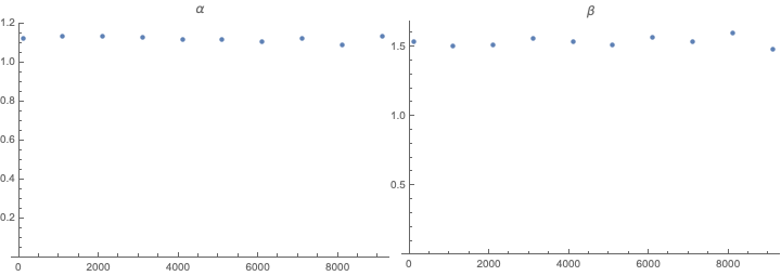
We can see that the parameters hardly vary and do not vary consistently with list length. We can then find parameters we like.
In[]:= $serialparams = \[Alpha]\[Beta]params[10000, 10000]
Out[]= {\[Alpha] -> 1.10793, \[Beta] -> 1.53947}

In[]:= $serialfitdist =
 GammaDistribution[\[Alpha], \[Beta]] /. $serialparams
Out[]= GammaDistribution[1.10793, 1.53947]
Our pvalue is then of the form:
1 - CDF[$serialfitdist, SerialTestStat[sequence]]
Discussion
This method is powerful as it examines the frequency and ordering of pairs. However, this method is contingent on one large assumptionthat the Wolfram Language pseudorandom number generator is truly pseudorandomor rather, that it is pseudorandom enough. A Monte Carlo approach is often very powerful for these sorts of statistics; however, it is important to be weary of such assumptions.
Runs tests
In these tests, we will investigate runs of both 0s and 1s and random reals between 0 and 1. A run is a sequence that fits a particular pattern until it is reset. For random reals, we will use increasing runs. For sequences of 0s and 1s, we obtain the runs by simply splitting the list:
How long are runs in a sequence?
The first statistic we will construct will measure the length of runs. Our approach will again utilize a Monte Carlo method. To measure runs:
runsup[seq_] := Split[seq, #1 < #2 &];
In order to count lengths of runs:
runLengthDist[seq_] := Length /@ runsup[seq]
The distribution of run lengths within a random sequence:
ListPlot[Counts@runLengthDist@RandomReal[{0, 1}, 1000000],
 Filling -> Axis]
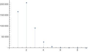
We can see that the run lengths quickly converge to a constant distribution. With this we can then calculate a constantthe mean run length:
In[]:= $meanRunLength =
 Mean[ParallelMap[ N@Mean[runLengthDist[#]] &,
   RandomReal[{0, 1}, {10000, 5000}]]]
Out[]:= 2.00004
We will then construct another chisquare like test statistic:
RunLengthStat[seq_] :=
  Total[(runLengthDist[seq] - $meanRunLength)^2/$meanRunLength];
This statistic turns out to be normally distributed with a mean and standard deviation associated with the sequence length. Putting all of this together, we can calculate the twotailed pvalue:
2 Min[{1 - CDF[##], CDF[##]}] &[
 NormalDistribution[runlength\[Mu][Length[sequence]],
  runlength\[Sigma][Length[sequence]]], RunLengthStat[sequence]];
where runlength\[Mu] and runlength\[Sigma] are determined empirically using the same method that was used to determine the parameters alpha and beta for the gamma distribution of the serial test.
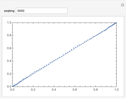
How many runs do we expect a sequence to have?
The next statistic we create will count the total amount of runs a sequence has. The statistic is then:
RunCountStat = Length[Split[#, (#1 < #2 &)]] &;
This distribution follows a normal distribution:
Manipulate[
 ProbabilityPlot[
  RunCountStat /@ RandomReal[{0, 1}, {1000, seqleng}]], {seqleng,
  5000}]
We can calculate and model the distribution using a MonteCarlo method to create a twotailed pvalue:
2 Min[{1 - CDF[##], CDF[##]}] &[
 NormalDistribution[runcount\[Mu][Length[sequence]],
  runcount\[Sigma][Length[sequence]]], RunCountStat[sequence]]
where
runcount\[Mu][seqleng_] = seqleng/2
runcount\[Sigma][seqleng_] = 0.303833 seqleng^0.493785
These formulae were developed using methods similar to those described in the section on serial testing.
How many runs does a sequence of zeros and ones have?
This test is taken entirely from an NIST publication. It only assesses sequences of 0s and 1s. Additionally, it is theoretically derived. The test statistic the publication gives is
NISTRunsstat = Length@Split@# &;
And the publication assigns the associated pvalue.
NISTRunspval =
  Erfc[Abs[Length@Split@#1 - 2 Length[#1] #2 (1 - #2)]/(
      2. Sqrt[2 Length[#1]] #2 (1 - #2))] &[#, Total[#]/Length[#]] &;
Spectral tests
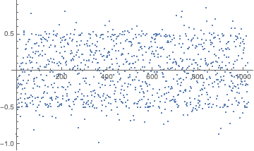
The spectral test will use the discrete cosine transform to assess the randomness of data. The transformed data should be homogeneous over frequency space and, overall, should be normally distributed. The transformed data should be normally distributed because the transformed data is obtained by:
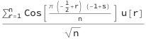
where u[r] is the rth random number in the sequence, s is the frequency parameter, and n is the length of the sequence. This can be reexpressed in the form:
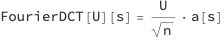
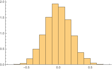
where U is the sequence, a[s] is a list of constants, and [CenterDot] is the dot product. This form tells us that each individual point is a sum of random variables. If these variables are truly independently and identically distributed, they should follow the normal distribution:
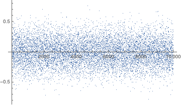
sequence = RandomReal[{0, 1}, 10000];
ListPlot[Rest@FourierDCT@sequence, PlotRange -> All]
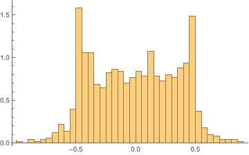
Histogram[Rest@FourierDCT@sequence, Automatic, "PDF"]
Our task then is to simply perform a KolmogorovSmirnov test for normality on the transformed data:
KolmogorovSmirnovTest[Rest@FourierDCT@sequence, Automatic, "PValue"]
Sequential sums tests
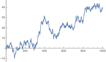
This test is entirely developed by the NIST publication. The test statistic for this test is based on the idea of generating a random walk from a list of zeros and ones. First, we transform the sequence and then accumulate the values.
sequence = RandomInteger[{0, 1}, 1000];
ListLinePlot[Accumulate[2 sequence - 1]]
For the statistic, we will look at the maximum distance away from zero that the walk obatins:
CUSUMmaxstat[seq_] := Max@Abs@Accumulate[2 seq - 1];
The stationary distribution is approximately normal. The publication uses this property to derive the following formula for the pvalue:
\[CapitalPhi][x_] = CDF[NormalDistribution[], x];
CUSUMmaxpval =
  Function[{z, n},
     1. - Sum[\[CapitalPhi][(z (4 k + 1))/Sqrt[n]] - \[CapitalPhi][(
         z (4 k - 1))/Sqrt[n]], {k, Floor[(-n/z + 1)/4], (n/z - 1)/4,
        1}] + Sum[\[CapitalPhi][(z (4 k + 3))/Sqrt[
         n]] - \[CapitalPhi][(z (4 k + 1))/Sqrt[n]], {k,
        Floor[(-n/z - 3)/4], (n/z - 1)/4, 1}]][CUSUMmaxstat[#],
    Length[#]] &;
Arcsine test
This test utilizes the arcsine law as described in Lorek, Los, Gotfryd, and Zagórski's publication. The arcsine law states that given a variable Xthe percentage of a random walk generated by a sequence of random reals spends above (or equivalently below) 0X will be distributed according to a particular 'arcsine distribution':
Table[Length@
   Cases[Accumulate[2 # - 1] &@RandomReal[{0, 1}, 1000], x_ /; x > 0]/
  1000, 10000];
Show[Histogram[%, 100, "CDF"],
 Plot[2/\[Pi] ArcSin[Sqrt[x]], {x, 0, 1}]]
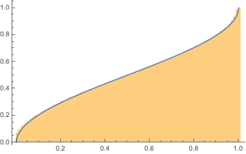
The formula for the CDF of the distribution is
$\text{CDF}[x]=\frac{2 \sin ^{-1}\left(\sqrt{x}\right)}{\pi }$
Our statistic is then the percentage of time a random walk generated from our sequence spends above 0:
Arcsinelawstat[seq_] :=
  Length@Cases[Accumulate[2 # - 1] &@seq, x_ /; x > 0]/Length[seq];
And we create a twotailed pvalue:
Arcsinelawpval[stat_] :=
  2 Min@{1 - #, #} &[2/\[Pi] ArcSin[Sqrt[stat]]];
Variates of arbitrary distributions
We can extend the scope of tests on sequences of random reals between 0 and 1. Using the property that the CDF of a distribution applied to its variates yield a uniform distribution, we can test the randomness of a sequence of variates from a known distribution. An example using the run length test:
variates = RandomVariate[NormalDistribution[], 10000];
transformedvariates = CDF[NormalDistribution[], variates]
.
ResourceFunction["RunLengthRandomnessTest"][transformedvariates, "TestStatistic"]
ResourceFunction["RunLengthRandomnessTest"][transformedvariates, "PValue"]
The pvalue should be uniformly distributed, ensuring the validity of the method.
Applications
Rule 30
Rule 30 is a cellular automaton rule introduced by Stephen Wolfram that was patented as a random number generator. At the alpha = .01 significance level, the center column of rule 30 passes all tests designed to test the randomness of sequences of 0s and 1s:
 A visualization of rule 30.
rule30seq =
  CellularAutomaton[30, {{1}, 0}, {10000, 0}]\[Transpose][[1]];

In[]:= ResourceFunction["ChiSquareRandomnessTest"][rule30seq]
Out[]:=0.515713
In[]:= ResourceFunction["ArcsineLawRandomnessTest"][rule30seq]
Out[]:=0.332579
In[]:= ResourceFunction["BinaryRunRandomnessTest"][rule30seq]
Out[]:=0.759777
In[]:= ResourceFunction["CUSUMaxRandomnessTest"][rule30seq]
Out[]:=0.370412
In[]:= ResourceFunction["SerialRandomnessTest"][rule30seq]
Out[]:=0.711583
In[]:= ResourceFunction["SpectralRandomnessTest"][rule30seq]
Out[]:=0.226717
Shift Register Sequences
We can also apply these tests to assess the randomness of shift register sequences. Shift registers are entities that generate sequences given certain internal characteristics. Shift registers are similar to cellular automata as they use feedback from previous sequence bits to create the next bit and. Shift registers can also be described using a characteristic polynomial. For this example, we will examine a maximallength linear shift register sequence:
shiftregistersequence = ShiftRegisterSequence[12];
 A visualization of a linear feedback shift register sequence
The shift register sequence passes several tests very well:
In[]:= ResourceFunction["ChiSquareRandomnessTest"][shiftregistersequence]
Out[]:=0.987532
In[]:= ResourceFunction["ArcsineLawRandomnessTest"][shiftregistersequence]
Out[]:=0.291655
In[]:= ResourceFunction["BinaryRunRandomnessTest"][shiftregistersequence]
Out[]:=0.987529
In[]:= ResourceFunction["CUSUMaxRandomnessTest"][shiftregistersequence]
Out[]:=0.567182
In[]:= ResourceFunction["SerialRandomnessTest"][shiftregistersequence]
Out[]:=0.997039
It is important to note that the sequence does seem to perform artificially highly on several tests. This observation is not cause to reject a hypothesis of randomness, but it is somewhat suspicious as it suggests that patterns within the generated sequence fit the expected patterns extremely well. While perform suspiciously well on some tests, the generated sequence horribly fails the spectral randomness test:
In[]:= ResourceFunction["SpectrallRandomnessTest"][shiftregistersequence]
Out[]:=0.
We can visualize how the discrete cosine transformed sequence fails to be normal, implying that observations are nonidentically and/or nonindependently distributed:
Histogram[Rest@FourierDCT@shiftregistersequence, 30, "PDF"]
ListPlot[Rest@FourierDCT@shiftregistersequence]
Conclusion
Summary
In this project we have successfully implemented 8 unique tests which evaluate both sequences of zeros and ones and sequences of reals between zero and one. The implemented tests are serial, run length, run count, chi square, spectral, KolmogorovSmirnov, cumulative sum, and arcsine law tests. Some tests are generated using a Monte Carlo method while others are theoretically derived. Some tests are implemented directly from methods published by NIST. The tests have additionally been applied to test the randomness of rule 30 and linear feedback shift registers; the randomness of rule 30 was not rejected while the randomness of a maximal linear feedback shift register was rejected.
Future directions
The scope of this project can be extended by implementing more testsspecifically tests that assess the entropy/information within a sequence. Some sequences fail certain tests but not others, so a unified conclusion describing the nature of the nonrandomness of a sequence is another possible direction. Including other measures of complexity of a sequence is another possible direction. Randomness, complexity, and information/entropy are all concepts that are deeply intertwined, so creating measures that reflect these concepts could be clarifying. Additionally, computational research into what an ideal alphavalue might be would be useful. Finally, one could also investigate the applications of randomness testing in more detail to assess systems like nonlinear feedback shift registers.
References
- NIST SP 800-22: Random Bit Generation
- [Lorek, Los, Gotfryd, Zagórski. On testing pseudorandom generators via statistical tests based on the arcsine law. arXiv:1903.09805.][34]
- Knuth, Donald E. The Art of Computer Programming. Third Edition, 1938.
 Attachments:


