Energy surface - Mathematica

I am working with a triaxial rigid rotor, which is a 3D object with no symmetry axis, so the moments of inertia about the principal axes are all different. It is well known from textbooks that the energy (rotational) of a triaxial rotor is given by the formula: $$E=A_1I_1^2+A_2I_2^2+A_3I_3^2\ ,$$ where the terms $A_k=\frac{1}{2\mathcal{I}_k}$ are the inverse of the moments of inertia $\mathcal{I}_k$, and $I_k$ represent the components of the total angular momentum $\mathbf{I}$.
My problem involves plotting the energy surface of the triaxial rotor, which should be a triaxial ellipsoid, deformed accordingly to the values of the inertia parameters $A_k$.

I chose to work in spherical coordinates, so a representation of the angular momentum vector using its components will be something like this: $$I_1\equiv x_1 =r\sin\theta\cos\varphi \\ I_2\equiv x_2=r\sin\theta\sin\varphi \\ I_3\equiv x_3=r\cos\theta$$ where $r\in[0,I]$ (can be any number but no larger than the maximum spin value $I$) , $\theta\in[0,\pi]$ (polar angle) and $\varphi\in[0,2\pi]$ (azimuthal angle).

The following arbitrary values for the inertia factors $A3=1$ , $A_1=6$, $A_2=3$, and the maximum spin $I=2$ are given. Note that the smallest inertia factor is the one corresponding to the 3-axis (so it means that the 3-axis has the largest moment of inertia). Therefore, choosing $x_3$ as the quantization axis is the right choice.

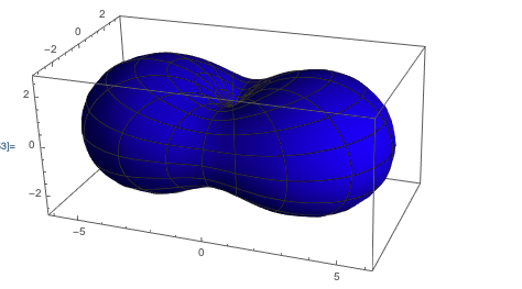
Now, for the graphical representation of the energy ellipsoid $E$, I was thinking of doing a SphericalPlot3D, since I work in spherical coordinates. Fixing $r$ to a value of $I=2$, and then trying to plot $E=f(r=I,\theta,\varphi)$, should (?) give me an ellipsoid. However, this is not what I obtain. The 3d object has some kind of neck. I don't understand why that is.

This is the code:

x1[r_, theta_, fi_] := r Sin[theta] Cos[fi]; 
x2[r_, theta_, fi_] := r Sin[theta] Sin[fi]; 
x3[r_, theta_, fi_] := r Cos[theta];

EnSphere[a1_, a2_, a3_, r_, theta_, fi_] := 
  a1*x1[r, theta, fi]^2 + a2*x2[r, theta, fi]^2 + 
   a3*x3[r, theta, fi]^2;

SphericalPlot3D[
 En3[A1, A2, A3, 1, \[Theta], \[Phi]], {\[Theta], 
  0, \[Pi]}, {\[Phi], 0, 2\[Pi]}, PlotStyle -> Blue]

This is what I obtain

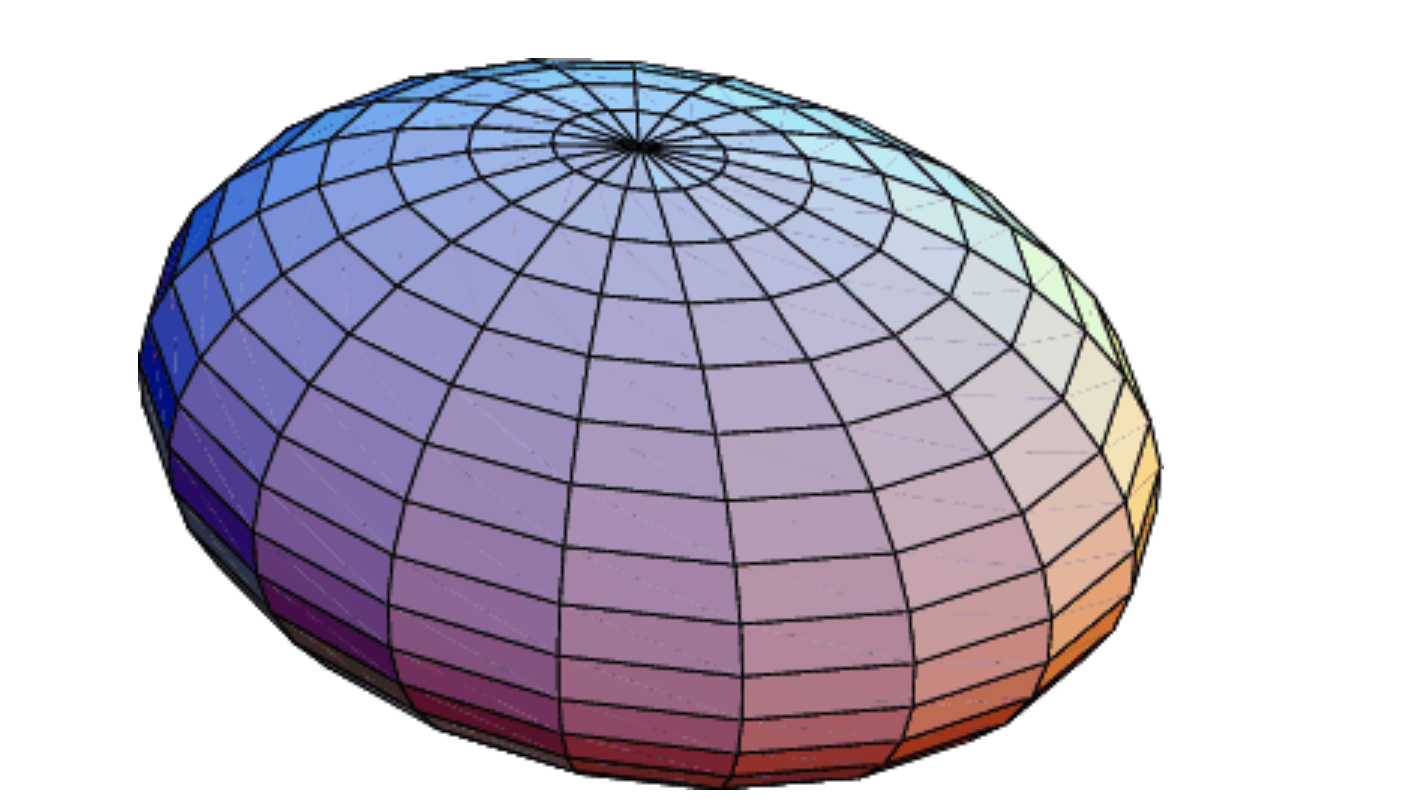
This is what I expected to obtain

Why is this happening? And how can I solve this? Is there a way to obtain the 3D energy surface of the triaxial rigid rotor starting from the values of the inertial parameters $A_k$?

Thank you in advance!