Vertex model is a special class of numerical simulations that is pervasively used in many areas of physics such as soft matter physics, engineering design, and more recently in developmental biology. For instance, classically in the soft matter community foams (Figure 1a) have usually been modeled by employing vertex model. Following a similar pursuit, biological tissues (Figure 1b) have also been simulated via vertex model. However, before I overwhelm the reader with the usage of the term, I would like to elucidate what exactly are vertex models?
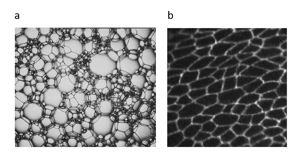 Figure 1 (a) dry foam (b) drosophila (fruitfly) epithelium
The tissues in our body are a collection of specialized cells that communicate with each other mechanically because cells are mechanically linked with each other. These cellular communities form a living system that perform work day and night by actively burning energy and preventing themselves from dying - or reaching thermodynamic equilibrium. If you are ever fortunate enough to observe a small slice of a tissue under an optical microscope, the membranes of the cells are constantly moving, flailing about in space and changing their length. As a result of coupled dynamic events cells can alter their morphology and configuration - oftentimes to perform specific functions e.g. think of the heart muscles that are perpetually relaxing and getting tensed in every beat.
Two dimensional and three-dimensional vertex models can be used to capture some of the dynamics of these active systems. In a two-dimensional setting, a foam or a biological tissue can be abstracted by a set of connected polygons (Figure 2). An edge of the polygon represents the edge of a bubble or a cell. It is through these network of edges(interfaces) that a bubble connects to its neighbouring bubble and likewise, the biological cells. Moreover, the ends of the edges constitute the vertices/junctions where more than two polygons meet. The movement of the vertices and consequently the edges can capture - in an abstract manner - the motion of the cell membranes and the dynamic behaviour of the cellular communities. Broadly we can take advantage of the vertex model to simulate a monolayer of cells (epithelia) or even an agglomerate of cells (e.g. a multilayered tissue).
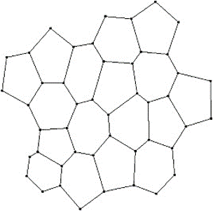
Figure 2: cells represented as polygons with shared edges (lines) and vertices (dots)
Simply putting the vertices are assumed to obey the following physical equation:
η dr/dt=-∇U
where η is the resistive coefficient, U is potential energy and r is the position vector associated with the vertex.
The vertices are displaced by virtue of the forces acting on them, with the forces generated as a result of the gradient of potential energy at that point. The potential energy can be a sum or contributions of multiple terms, with the more notable being the spring energy terms associated with changes in cell area, perimeter etc... Keeping the above equation in view, the vertices will move down the gradient in a deterministic fashion to minimize the total potential energy of the system. The relative motion of the vertices in space will eventually lead to newer topologies - topologies that are energetically more feasible. In a naïve manner we assume that this holds for biological cells where the relative or collective movement of cells in the community establish new tissue architectures that are also energetically favourable states. Moreover, we can infer a lot about the dynamics governing morphogenesis and animal development by looking at the forces, by extension the stresses, acting on the cells by utilizing vertex models. Additionally, one can also implement procedures in vertex model to emulate neighbourhood exchanges whereby a cell can switch its immediate neighbours.
In a three dimensional context each polygon is replaced by a polyhedron whilst the governing equations remain unaltered. The cells in 3D not only share edges but faces as well (Figure 3). In this post, I am releasing the first versions of my notebooks. For notebooks please visit the github repository 3D-Vertex-Model. I will discuss how the fascinating new capabilities of Mathematica 12.1 especially for computational geometry can allow us to construct the more complex 3D vertex models. Though I must admit that the implementation of the 3D vertex model was a somewhat long and dauting task. The implementation is based of the approach presented in "Reversible network reconnection model for simulating large deformation in dynamic tissue morphogenesis", (Biomechanics and modeling in Mechanobiology 2013). As is mostly the case the authors have not released the code to the public. I do not know why this is the case when all the code should be released on both scientific and ethical grounds. But that is entirely a different rant.
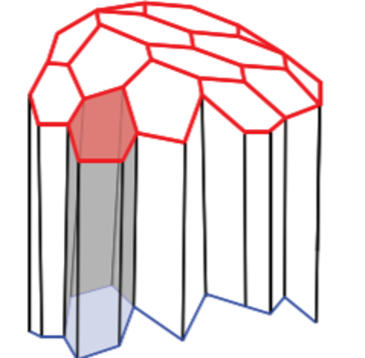
Figure 3: in three dimensions cells share edges and faces with their neighbours
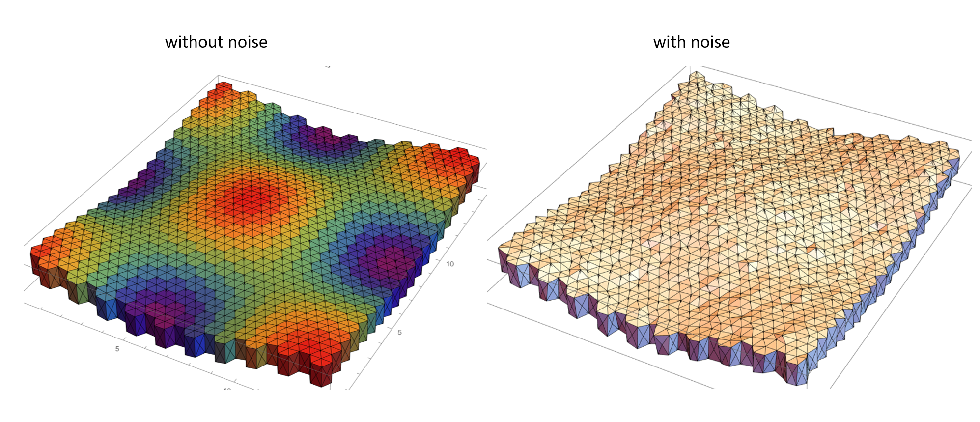
I started constructing the 3D vertex model in version 12.0 however along the way 12.1 came and I tweaked the code a bit to take advantage of the additional capabilities of version 12.1. For the purpose of this post my aim is to model an infinite sheet (epithelium) of cells. The infinite aspect is established by ensuring periodic boundary conditions at the edges of the simulation domain. Nevertheless, the code can be conveniently tweaked to model a multilayered system such as a cluster of cells. The quintessential ingredients of the vertex model includes a geometric mesh and a choice of a numerical solver to propagate the vertices. A polyhedra sheet is established by the following recipe. The vertices for the polygons are setup spatially as a two dimensional curved sheet which are mirrored in the z direction. The two layers of polygons are connected laterally to create the third dimension. Thereafter a Polyhedron function is applied to a single cell to create a hexahedral prism (below) and their collection forms the prism lattice.
The cells at the edges of the simulation domain are stitched together to ensure periodic boundary conditions. The vertices are displaced slightly from their initial configuration by sampling noise from a normal distribution. Yet again, a periodic boundary condition is ensured at the edges of the mesh. The noise can be thought of as a perturbation from the stable hexahedral prism lattice configuration and infuses the mesh with higher energy. "infinite-sheet".nb and "infinite sheet - noise addition".nb make extensive use of built-in Mathematica functionality and custom routines to generate the curved hexahedral prism lattice and add noise to the vertices in the mesh respectively. The geometric mesh prior to and with the addition of noise are depicted below.
Once the mesh is created we now require a numerical procedure to solve for the vertex displacement. I have implemented a Runge-Kutta 5th order numerical integration scheme which allows me to use a relatively larger timestep without a loss in numerical accuracy when compared to say Heun's integrator. The potential energies considered in the study can be decomposed into two parts; a part associated with surfaces (between cells and those between cells and the outside, where the outside can be some liquid) and a second contribution owing to the volumetric elasticity of the cells away from an equilibrium value. The gradient of the potential energy term is determined by taking the gradient of the surface energy and the volumetric energy terms. And this is where Mathematica 12.1 shines ! The new computational geometry features coupled with a lot of custom (CompiledC, and Listable) routines from discrete differential geometry allow me to evaluate these terms quite conveniently.
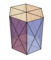
Additionally we can include some kind of transformation rules that instruct the cells when and how to exchange their neighbours. The neighbour exchanges in this model can take place by considering two types of transitions: a shared edge between two cells - smaller than a defined threshold- is replaced by a trigonal face, and the process is reversible. Consider a set of four polyhedrons (Figure 4); a network transformation rule (I-to-∆, see the journal article) allows the polyhedrons to swap neighbours by eliminating an edge and establishing a new trigonal face between cells. Another transformation rule (not shown here) takes a small trigonal face between cells and establishes a new edge in lieu of a face.
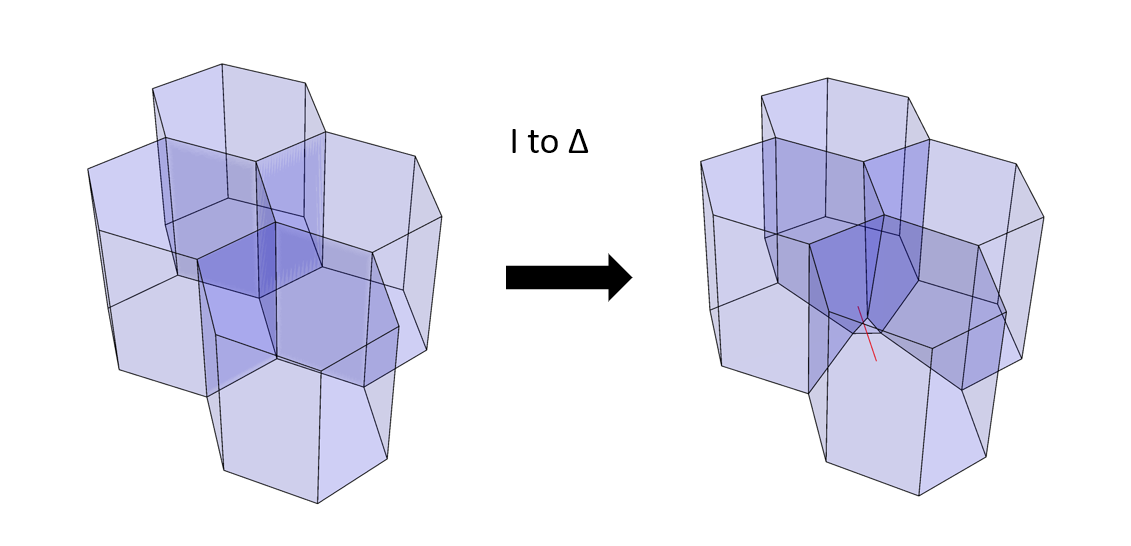
Figure 4: a type of network transformation that changes the cell neighbourhood
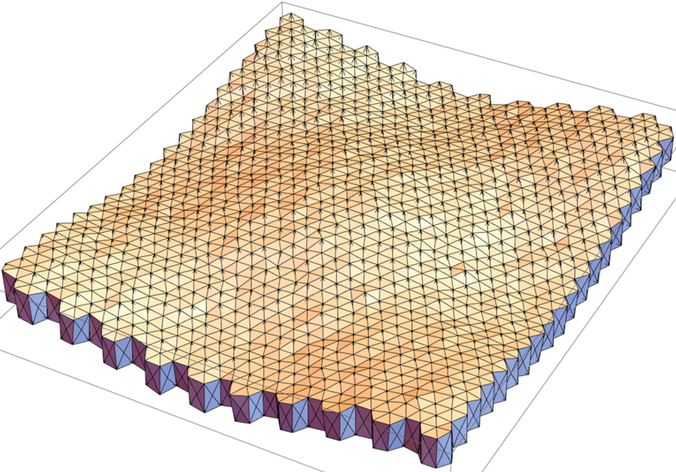
The numerical integration scheme and the topological transition rules (neighbourhood exchanges) are included in "vertex model 3D".nb. The mesh created from the earlier notebooks is imported into it. Some polyhedral cells in the mesh are labelled as "growing" (with active increase in size) whereas the majority of the cells are non-growing (no active increase in volume). The mesh is then integrated over time. The result for the current mesh (400 cells) after a few integration steps is shown below.
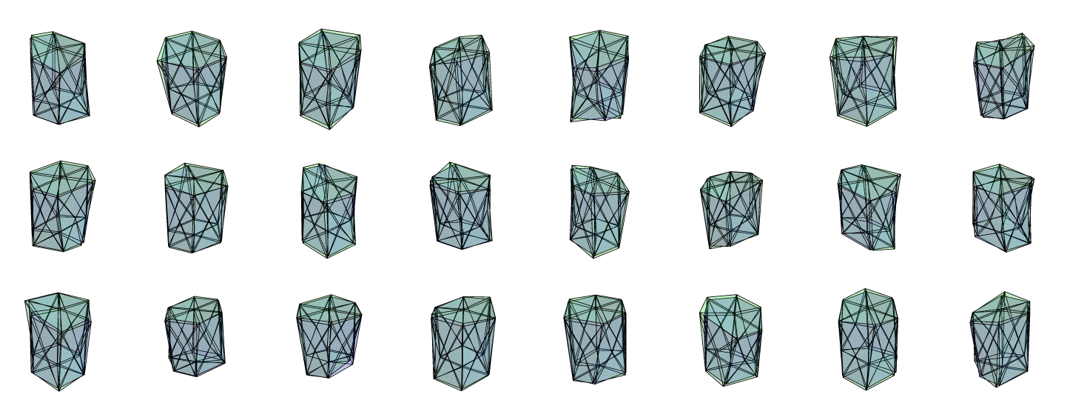
The initial state (prior to iterations) and the final states (post iterations) of a few cells can be superimposed to note for the changes.
Although I have not had the time to run it as of yet, I have computed that it will take approximately a month to generate the results that the authors have presented in their study. I will do that soon. Well 30 days is quite less in the span of a human lifetime and provided there is an extra computer to spare. Also while I am at it I will remember the proverb "a watched pot never boils" and stick to it :)
I hope that my post shows that computational geometry is not just relevant for experts working with Graphics and Finite Elements, but also for people like me who are trying to understand biological phenomena using physical principles.
The entire code is a bit too elaborate to paste here directly and I do not intend to overwhelm anyone reading the post as I want to keep it bare-bones. Nevertheless, I have utilized nearly all programming paradigms that Mathematica has to offer; a mix of rule-based substitutions, functional and procedural programming are all applied wherever their specific need arose. Yet there are a couple of code excerpts that I will paste here as they prove to be quite important:
I particularly love this portion mainly because of the simplicity: this is how I created polyhedra from two curved surfaces
initFace = {{1, 2, 3, 4, 5, 6}, {7, 12, 11, 10, 9, 8},
   Sequence @@ NestList[# + 1 &, {1, 7, 8, 2}, 4], {6, 12, 7, 1}};
faceListInd = NestList[# + 12 &, initFace, (cellNumX*cellNumX) - 1];
faceListCoords = MapAt[Lookup[indToPtsAssoc, #] &, faceListInd, {All, All, All}];
you can view say the first polyhedron that has triangulated faces as:
firstPolyhedra = First@faceListCoords;
Graphics3D[{Directive[Blue, Opacity[0.25*1/GoldenRatio]],Polyhedron@Flatten[triangulateFaces[firstPolyhedra], 1]
the triangulateFaces function is as follows:
Triangulation of faces of polyhedra
Clear[triangulateFaces];
triangulateFaces::Information = "the f(x) takes in cell faces and triangulates them";
triangulateFaces[faces_] := Block[{edgelen, ls, mean},
(If[Length[#] ≠ 3,
ls = Partition[#, 2, 1, 1];
edgelen = Norm[SetPrecision[First[#] - Last[#], 8]] & /@ ls;
mean = Total[edgelen * (Midpoint /@ ls)] / Total[edgelen];
mean = mean~SetPrecision~8;
Map[Append[#, mean] &, ls],
{#}
]) & /@ faces];
to find local neighbourhood of a vertex or an edge I have devised the following rules and functions. They also work for vertices at the edge of the simulation domain as I ensure periodic boundary conditions:
rules to find neighbourhood given periodic boundary conditions
periodicRules::Information =
  "shift the points outside the simulation domain to inside the domain";
transformRules::Information =
  "vector that shifts the point outside the simulation domain back inside";
With[{xlim1 = xLim[[1]], xlim2 = xLim[[2]], ylim1 = yLim[[1]],
   ylim2 = yLim[[2]]},
  periodicRules = Dispatch[{
     {x_ /; x >= xlim2, y_ /; y <= ylim1, z_} :>
      SetPrecision[{x - xlim2, y + ylim2, z}, 8],
     {x_ /; x >= xlim2, y_ /; ylim1 < y < ylim2, z_} :>
      SetPrecision[{x - xlim2, y, z}, 8],
     {x_ /; xlim1 < x < xlim2, y_ /; y <= ylim1, z_} :>
      SetPrecision[{x, y + ylim2, z}, 8],
     {x_ /; x <= xlim1, y_ /; y <= ylim1, z_} :>
      SetPrecision[{x + xlim2, y + ylim2, z}, 8],
     {x_ /; x <= xlim1, y_ /; ylim1 < y < ylim2, z_} :>
      SetPrecision[{x + xlim2, y, z}, 8],
     {x_ /; x <= xlim1, y_ /; y >= ylim2, z_} :>
      SetPrecision[{x + xlim2, y - ylim2, z}, 8],
     {x_ /; xlim1 < x < xlim2, y_ /; y >= ylim2, z_} :>
      SetPrecision[{x, y - ylim2, z}, 8],
     {x_ /; x >= xlim2, y_ /; y >= ylim2, z_} :>
      SetPrecision[{x - xlim2, y - ylim2, z}, 8]
     }];

  transformRules = Dispatch[{
     {x_ /; x >= xlim2, y_ /; y <= ylim1, _} :>
      SetPrecision[{-xlim2, ylim2, 0}, 8],
     {x_ /; x >= xlim2, y_ /; ylim1 < y < ylim2, _} :>
      SetPrecision[{-xlim2, 0, 0}, 8],
     {x_ /; xlim1 < x < xlim2, y_ /; y <= ylim1, _} :>
      SetPrecision[{0, ylim2, 0}, 8],
     {x_ /; x <= xlim1, y_ /; y <= ylim1, _} :>
      SetPrecision[{xlim2, ylim2, 0}, 8],
     {x_ /; x <= xlim1, y_ /; ylim1 < y < ylim2, _} :>
      SetPrecision[{xlim2, 0, 0}, 8],
     {x_ /; x <= xlim1, y_ /; y >= ylim2, _} :>
      SetPrecision[{xlim2, -ylim2, 0}, 8],
     {x_ /; xlim1 < x < xlim2, y_ /; y >= ylim2, _} :>
      SetPrecision[{0, -ylim2, 0}, 8],
     {x_ /; x >= xlim2, y_ /; y >= ylim2, _} :>
      SetPrecision[{-xlim2, -ylim2, 0}, 8],
     {___Real} :> SetPrecision[{0, 0, 0}, 8]}];
  ];

(*wrappedMat =
    AssociationThread[
     Keys[cellVertexGrouping] ->
      Map[Lookup[indToPtsAssoc, #] /. periodicRules &,
       Lookup[cellVertexGrouping, Keys[cellVertexGrouping]], {2}]];*)
and one can find local topology by getLocalTopology
getLocalTopology[ptsToIndAssoc_, indToPtsAssoc_, vertexToCell_,
    cellVertexGrouping_, wrappedMat_, faceListCoords_][vertices_] :=
  Block[{localtopology = <||>, wrappedcellList = {}, vertcellconns,
    localcellunion, v, wrappedcellpos, vertcs = vertices, rl1, rl2,
    transVector, wrappedcellCoords, wrappedcells, vertOutofBounds,
    shiftedPt, transvecList = {}, $faceListCoords = Values@faceListCoords,
    vertexQ, boundsCheck, rules, extractcellkeys, vertind,
    cellsconnected, wrappedcellsrem},
   vertexQ = MatchQ[vertices, {__?NumberQ}];
   If[vertexQ,
    (vertcellconns =
      AssociationThread[{#} , {vertexToCell[ptsToIndAssoc[#]]}] &@
       vertices;
     vertcs = {vertices};
     localcellunion = Flatten[Values@vertcellconns]),
    (vertcellconns =
      AssociationThread[# ,
         Lookup[vertexToCell, Lookup[ptsToIndAssoc, #]]] &@vertices;
     localcellunion = Union@Flatten[Values@vertcellconns])
    ];

   If[localcellunion != {},
    AppendTo[localtopology,
     Thread[
      localcellunion ->
       Map[Lookup[indToPtsAssoc, #] &,
        cellVertexGrouping /@ localcellunion, {2}]]
     ]
    ];
   (* condition to be an internal edge: both vertices should have 3 neighbours *)
   (* if a vertex has 3 cells in its local neighbourhood then the \
entire network topology about the vertex is known \[Rule] no wrapping required *)
   (* else we need to wrap around the vertex because other cells are \
connected to it \[Rule] periodic boundary conditions *)
   With[{vert = #},
      vertind = ptsToIndAssoc[vert];
      cellsconnected = vertexToCell[vertind];
      If[Length[cellsconnected] != 3,
       If[(\[ScriptCapitalD]~RegionMember~Most[vert]),
         (*Print["vertex inside bounds"];*)
         v = vert;
         With[{x = v[[1]], y = v[[2]]},
          boundsCheck = (x == xLim[[1]] || x == xLim[[2]] ||
             y == yLim[[1]] || y == yLim[[2]])];

         extractcellkeys = If[boundsCheck,
           {rl1, rl2} = {v, v /. periodicRules};
           rules = Block[{x$},
             With[{r = rl1, s = rl2},
              DeleteDuplicates[
               HoldPattern[SameQ[x$, r]] || HoldPattern[SameQ[x$, s]]]
              ]
             ];
           Position @@ With[{rule = rules},
             Hold[wrappedMat, x_ /; ReleaseHold@rule, {3}]
             ],
           Position[wrappedMat, x_ /; SameQ[x, v], {3}]
           ];
         (*
         find cell indices that are attached to the vertex in wrappedMat *)
         wrappedcellpos = DeleteDuplicatesBy[
           Cases[extractcellkeys,
            {Key[
               p : Except[
                 Alternatives @@
                  Join[localcellunion, Flatten@wrappedcellList]]],
              y__} :> {p, y}],
           First];
         (*wrappedcellpos = wrappedcellpos/.{Alternatives@@Flatten[
         wrappedcellList],__} \[RuleDelayed] Sequence[];*)
         (* if a wrapped cell has not been considered earlier (i.e. is new) then
we translate it to the position of the vertex *)

         If[wrappedcellpos != {},
          If[vertexQ,

           transVector =
            SetPrecision[(v -
                 Extract[$faceListCoords,
                  Replace[#, {p_, q__} :> {Key[p], q}, {1}]]) & /@
              wrappedcellpos, 8],
           (* call to function is enquiring an edge and not a vertex*)

           transVector =
            SetPrecision[(v - Extract[$faceListCoords, #]) & /@
              wrappedcellpos, 8]
           ];

          wrappedcellCoords =
           MapThread[#1 ->
              Map[Function[x, SetPrecision[x + #2, 8]], $faceListCoords[[#1]], {2}] &,
            {First /@ wrappedcellpos, transVector}];
          wrappedcells = Keys@wrappedcellCoords;
          AppendTo[wrappedcellList, Flatten@wrappedcells];
          AppendTo[transvecList, transVector];
          AppendTo[localtopology, wrappedcellCoords];
          ],
         (* the else clause: vertex is out of bounds *)
         (*Print["vertex out of bounds"];*)
         vertOutofBounds = vert;
         (* translate the vertex back into mesh *)
         transVector = vertOutofBounds /. transformRules;
         shiftedPt = SetPrecision[vertOutofBounds + transVector, 8];
         (* ------------- CORE B ------------- *)
         (*
         find which cells the shifted vertex is a part of in the \
wrapped matrix *)
         wrappedcells = Complement[

           Union@Cases[
              Position[wrappedMat, x_ /; SameQ[x, shiftedPt], {3}],
              x_Key :> Sequence @@ x, {2}] /.
            Alternatives @@ localcellunion -> Sequence[],
           Flatten@wrappedcellList];

         (*forming local topology now that we know the wrapped cells *)


         If[wrappedcells != {},
          AppendTo[wrappedcellList, Flatten@wrappedcells];
          wrappedcellCoords = AssociationThread[wrappedcells,
            Map[Lookup[indToPtsAssoc, #] &,
             cellVertexGrouping[#] & /@ wrappedcells, {2}]];
          With[{opt = (vertOutofBounds /. periodicRules)},
           Block[{pos, vertref, transvec},
             Do[
              With[{cellcoords = wrappedcellCoords[cell]},
               pos = FirstPosition[cellcoords /. periodicRules, opt];
               vertref = Extract[cellcoords, pos];
               transvec = SetPrecision[vertOutofBounds - vertref, 8];
               AppendTo[transvecList, transvec];

               AppendTo[localtopology,
                cell ->
                 Map[SetPrecision[# + transvec, 8] &,
                  cellcoords, {2}]];
               ], {cell, wrappedcells}]
             ];
           ];
          ];
         (* to detect wrapped cells not detected by CORE B*)
         (* ------------- CORE C ------------- *)
         Block[{pos, celllocs, ls, transvec, assoc, tvecLs = {}, ckey},
          ls = Union@Flatten@Join[cellsconnected, wrappedcells];
          If[Length[ls] != 3,

           pos = Position[faceListCoords, x_ /; SameQ[x, shiftedPt], {3}];

           celllocs =
            DeleteDuplicatesBy[
              Cases[pos, Except[{Key[Alternatives @@ ls], __}]],
              First] /. {Key[x_], z__} :> {Key[x], {z}};
           If[celllocs != {},
            celllocs = Transpose@celllocs;
            assoc = <|
              MapThread[
               (transvec =
                  SetPrecision[
                   vertOutofBounds -
                    Extract[faceListCoords[Sequence @@ #1], #2], 8];
                 ckey = Identity @@ #1;
                 AppendTo[tvecLs, transvec];

                 ckey ->
                  Map[SetPrecision[
                    Lookup[indToPtsAssoc, #] + transvec, 8] &,
                   cellVertexGrouping[Sequence @@ #1], {2}]
                 ) &, celllocs]
              |>;
            AppendTo[localtopology, assoc];
            AppendTo[wrappedcellList, Keys@assoc];
            AppendTo[transvecList, tvecLs];
            ];
           ];
          ];
         ];
       ];
      ] & /@ vertcs;

   transvecList = Which[
     MatchQ[transvecList, {{{__?NumberQ}}}], First[transvecList],
     MatchQ[transvecList, {{__?NumberQ} ..}], transvecList,
     True,
     transvecList //. {x___, {p : {__?NumberQ} ..}, y___} :> {x, p, y}
     ];
   {localtopology, Flatten@wrappedcellList, transvecList}
   ];
The small excerpts from the code for the computation of surface gradient and volumetric gradient are as follows:
SurfaceGradient
ClearAll@surfaceGrad;
surfaceGrad::Information =
"surfaceGrad takes in arguments and computes the surface gradient about a point";
With[{epcc = ϵcc, epco = ϵco},
surfaceGrad = Compile[{{point, _Real, 1}, {opentr, _Real, 3},
{normalO, _Real, 2}, {closedtr, _Real, 3}, {normalC, _Real, 2}},
Block[{ptTri, source = point, normal, target, facept, cross,
openS = {0., 0., 0.}, closedS = {0., 0., 0.}},
Do[
ptTri = opentr[[i]];
normal = normalO[[i]];
cross = If[Chop[ptTri[[1]] - source, 10^-8] ⩵ {0., 0., 0.},
{target, facept} = {ptTri[[2]], ptTri[[-1]]};
Cross[normal, facept - target],
{target, facept} = {ptTri[[1]], ptTri[[-1]]};
Cross[normal, target - facept]
];
openS += (0.5 * cross), {i, Length@normalO}];
Do[
ptTri = closedtr[[j]];
normal = normalC[[j]];
cross = If[Chop[ptTri[[1]] - source, 10^-8] ⩵ {0., 0., 0.},
{target, facept} = {ptTri[[2]], ptTri[[-1]]};
Cross[normal, facept - target],
{target, facept} = {ptTri[[1]], ptTri[[-1]]};
Cross[normal, target - facept]
];
closedS += (0.5 * cross), {j, Length@normalC}];
epcc * closedS + epco * openS], CompilationTarget → "C", RuntimeOptions → "Speed",
CompilationOptions →
{"ExpressionOptimization" → True, "InlineExternalDefinitions" → True}]
VolumeGradient
Clear@volumeGrad;
volumeGrad::Information = "volumeGrad computes the volume gradient about a point";
volumeGrad[normalsAssoc_, cellids_, assocTri_, polyhedVols_, growingCellIds_] :=
Block[{celltopology, gradV, vol, growindkeys},
gradV = With[{nA = normalsAssoc, aT = assocTri},
Table[
celltopology = aT[cell];
(1. / 3.) Total[(areaTriFn[#] × nA[#]) & /@ celltopology], {cell, cellids}]
];
vol = AssociationThread[cellids → ConstantArray[Vo, Length@cellids]];
growindkeys =
Replace[Intersection[cellids, growingCellIds], k_Integer ⧴ {Key[k]}, {1}];
vol = Values@If[growindkeys ≠ {}, MapAt[(1 + Vgrowth time) # &, vol, growindkeys], vol];
kcv Total[((polyhedVols/vol) - 1) gradV]
];
Overall I am quite impressed by the latest versions of Mathematica. Something of this sort in my opinion was not possible before version 12. And so the computational geometry features are a welcome addition to the already extensive capabilities of Mathematica. I hope people at Wolfram keep adding more and more features for computational geometry in the upcoming versions for Mathematica.
Note 1: In "vertex model 3D".nb I have tried to incorporate some simple schemes to detect and prevent collision of polyhedral cells. Theoretically, the polyhedrons can possibly intersect each other but in reality we know that cells are not ghosts. I hope that in the future release of Mathematica some built-in fast functions for computational geometry can be incorporated to determine if two or more polyhedral objects are colliding or intersecting.
Note 2: The topological transition rule relies on a check - SubIsomorphicQ function from Szabolcs Horvat's brilliant IGraphM package.
Note 3: I have plans to expand the functionality in future by incorporating divisions and removal of polyhedrons in the mesh, in a manner mimicking biological cell division and death. Plus other functionalities will hopefully follow. If you have any interest in talking to me or wanting to contribute or optimise the code, please feel free to contact me.
References for figures:
Figure 1a: https://www.researchgate.net/figure/Photograph-of-a-typical-dry-foam-a-close-packing-of-bubbles-of-a-wide-distribution-of_fig1_265117106
Figure 1b: https://www.researchgate.net/figure/a-left-Confocal-microscope-image-of-a-developing-Drosophila-wing-E-cadherin-labelled_fig1_47809672
Figure 2: https://www.sciencedirect.com/science/article/pii/S0079610713000989
Figure 3: https://royalsocietypublishing.org/doi/pdf/10.1098/rstb.2015.0520
 Attachments:


