Message Boards Message Boards

1
|
4748 Views
|
8 Replies
|
2 Total Likes
View groups...
Share
Share this post:

Using NBodySimulation with a custom pairwise function?

Posted 2 years ago

Background:

Popular solid-state Nuclear Magnetic Resonance (NMR) techniques measure inter-atomic distances by observing the rate of transfer of magnetization between two spins by a spin diffusion mechanism. Plots of normalized magnetization vs spin diffusion mixing time are matched with simulated spin diffusion buildup curves for various inter-atomic distances (r) to find the best fit.

For some interesting biomolecular problems, such as the distance from membrane lipids chains to a site on a protein, the following 1D lattice simulation procedure is implemented:

  1. Arrange (r+1) points i along a 1D grid with width equal to your "guess" distance r.
  2. Set initial magnetization: M1,t=0 = 1 and Mi=/=1, t=0 = 0
  3. Evolve magnetization for all points by ∆Mi/∆t = D/a2[(Mi+1 - Mi) - (Mi - Mi-1)] (where D and a2 are constants) for some # of steps.
  4. Repeat for different simulation times and make a buildup curve; determine fit with data.

Question How do I implement Step 3 above in the law argument of the NBodySimulation function? Follow-up question if this is impossible: Should I be going a SystemModelParametricSimulate direction instead?

Note: this Mathematica Stack Exchange thread ends with a similar unanswered query: https://mathematica.stackexchange.com/questions/105342/how-best-to-simulate-n-body-systems-in-a-functional-way

8 Replies

Update post

Hi all,

Thank you so much for taking a crack at this!! There are a few complicating factors I abridged out of the original post for brevity. For example, I'm going to be dealing with spin diffusion across material interfaces, i.e. the edge of a membrane in contact with water, and therefore there will be different values of the diffusivity D/a^2 at different points on the grid. This is no big deal to implement though. I have begun coding a solution inspired by all of yours (@Hans Dolhaine; @Henrik Schachner; Joshua Schrier), that basically iteratively operates on the 1D magnetization. I have had to reach out to the author of the FORTRAN code I'm trying to replicate to ask a few questions about the setup, and am waiting for a reply. When I (hopefully, God willing) finish a full solution, I will verify some prior experimental results and make a new Community Forum post and link it here.

Also, sorry for the delay. In my defense, I'm writing my doctoral thesis and this probably won't make it in; it's a for-the-joy-of-it endeavor!

Gratefully,

Madeleine Sutherland

Hello Madeleine,

thank you for you thank you. That is kind.

Concerning the diffusion in two phases : Long time ago I wrote a code dealing with that problem. Perhaps it is helpful.

a = 2.; b = 6; du = .1; dv = .8; u0 = 5.; v0 = 1.5;ux = 1/a; vx = 1/(a - b);

Clear[sol]
sol[t1_] := Module[{},
  {g, h} /. NDSolve[
     {
      D[ g[x, t], t] == ux^2 du  D[g[x, t], x, x],
      D[ h[x, t], t] == vx^2 dv D[ h[x, t], x, x],
      g[x, 0] == u0,
      h[x, 0] == v0,
      (D[ g[x, t], x] == 0) /. x -> 0,
      (D[ h[x, t], x] == 0) /. x -> 0,
      (  ux  du D[ g[x, t], x] == vx  dv D[h[x, t], x]) /. x -> 1,
      h[1, t] == g[1, t] (1 - Exp[-30 t]) + v0 Exp[-30 t]
      },
     {g, h},
     {x, 0, 1}, {t, 0, t1}][[1]]
  ]

lsg = sol[20];
f1 = lsg[[1]];
f2 = lsg[[2]];

fp[x_, t_] := If[x < a, f1[x/a, t], f2[(x - b)/(a - b), t]]

Manipulate[
 Plot[fp[x, tt], {x, 0, b}, PlotRange -> {0, 6}],
 {tt, 0, 20}]

And good luck for your thesis.

POSTED BY: Hans Dolhaine

Dear all,

I do hope that this is not off-topic, but I would like to make the remark that when the evolution of magnetization is described by the respective differential equation (instead of a difference equation), this system can be solved in an analytic way easily:

dim = 10;  (* number of magnets: *)
(* definition of the before mentioned "update matrix": *)
mat = Normal@
   SparseArray[{Band[{1, 1}] -> -2, Band[{1, 2}] -> 1, Band[{2, 1}] -> 1}, {dim, dim}];
mat[[1, 1]] = mat[[dim, dim]] = -1;
mat // MatrixForm

Then we have equation : d magVec / dt == mat.magVec, and mat.magVec gives the desired terms (all constants are set to 1) :

(* general magnetic vector: *)
magVec = Table[m[n], {n, 1, dim}];
(* 'd/dt' on lhs is just "symbolic" to show the system of equations! *)
Thread[(d /dt) magVec == mat.magVec] // MatrixForm
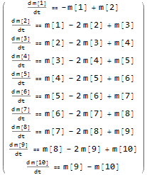
enter image description here

(* solution matrix in time 't': Exp[mat t], i.e.: *)
expMat = MatrixExp[mat  t];
(* initial condition - magnetic state at t==0: *)
startMagnVect = Prepend[ConstantArray[0, dim - 1], 1];
(*  {1, 0, 0, 0, 0, 0, 0, 0, 0, 0}  *)
(* analytical solution: *)
mgt = expMat.startMagnVect;
mgtN = N[mgt];

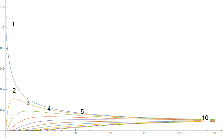
Plot of the result, i.e. magnetization in time:

labels = Style[#, 20] & /@ Range[dim];
Plot[mgtN, {t, 0, 30}, ImageSize -> 600, PlotRange -> All, PlotLabels -> Placed[labels, Above]]
enter image description here

The sum of all solutions is alway '1' - as correctly claimed by @Hans Dolhaine :

Total@mgt // Simplify
(* Out:    1 *)

And all limits seem to be the same - consequently '1/dim', e.g.:

Limit[mgt[[4]], t -> Infinity]
(* Out:   1/10   *)

The dimensionality of this method is quite limited; if you go beyond dim = 10; the calculation time explode. But it seems to show the general behaviour, though.

POSTED BY: Henrik Schachner

Hello Joshua,

that looks intriguing, but: the equation given by Madeline (point 3 above) is a diffusion equation, so Total/@results should always give one. This at least is the case with mm[i] calculated in my code above. What is going wrong?

POSTED BY: Hans Dolhaine

I suspect it might be related to the boundary conditions...there is a non-conservation at the boundaries because of the interpretation of how to treat the (Mi-1 - Mi) term when i=1. (this can be seen by doing a MatrixForm@update[10, 0.1]). My reading of @MadeleineSutherland's post was that the i-1 term can be discarded, while retaining the i term...but maybe that's not such a physically appropriate idea. Modifying the ends of the matrix to remove these terms should suffice.

POSTED BY: Joshua Schrier

Yes, this does the job

update2[r_Integer, constants_] := constants*Table[
   If[
    (i != 1 + r || j != 1 + r) && (i != 1 || j != 1),
    (KroneckerDelta[i + 1, j] - 
       KroneckerDelta[i, j]) - (KroneckerDelta[i, j] - 
       KroneckerDelta[i - 1, j]),
    -1]
   , {i, r + 1}, {j, r + 1}]
POSTED BY: Hans Dolhaine

To answer the original question: the documentation for NBodySimulation seems to suggest that only position changes are allowed, which would preclude using it for a problem like this.

You could also write this in a functional style (avoiding the use of Do loops) like the following. This is equivalent to @HansDolhaine's first solution above:

    initialState[r_Integer] := {1}~Join~ConstantArray[0, r] 

(*  define a matrix to perform the update step; for large systems, consider using SparseArray*)
(* lump all constants together*)
    update[r_Integer, constants_] := constants*Table[
       (KroneckerDelta[i + 1, j] - KroneckerDelta[i, j]) - (KroneckerDelta[i, j] -KroneckerDelta[i - 1, j]),
     {i, r + 1}, {j, r + 1}]

(*compute a lists of states at each tilmestep*)
results = With[
   {start = initialState[10],
    step = update[10, 0.1],
    timesteps = 20},
   NestList[ (step . # + #) &, start, timesteps]];

ArrayPlot[results] (*watch the magnitization*)

ListLinePlot[Mean /@ results] (*compute properties at each timestep and plot*)
POSTED BY: Joshua Schrier

Hello Madeleine,

perhaps something like this?

coeff = .4;  (* "Diffusion" constant *)
nS = 100;        (* number of sites *)
nT = 150;    (* number of time - steps  *)
m = Table[0, {nS}]; m[[1]] = 1;  (* magnetisation  *)
dd = m;  (* change of magnetization  *)
nc = 1;
mm[nc] = m;
While[
 nc <= nT,
 Do[
  Which[
   1 < i < nS, nv = coeff (m[[i + 1]] - 2 m[[i]] + m[[i - 1]]),
   i == 1, nv = coeff (m[[2]] - m[[1]]); dd[[1]] = nv,
   i == nS - 1, nv = coeff (m[[nS - 1]] - m[[nS]]); dd[[nS]] = nv
   ];
  dd[[i]] = nv,
  {i, 1, nS}
  ];
 nc = nc + 1;
 m = m + dd;
 (*Print[m];*)
 mm[nc] = m]

Manipulate[
 ListLinePlot[mm[nn], PlotRange -> {0, 1}],
 {nn, 1, nT, 1}]

Note that 0<= coeff < .5 is a must, otherwise you get a strange behavior (oscillations).

Your basic equation ( change of magnetization ) evokes the idea of a diffusion- process.

Therefore you can consider something like this. The warning "mxsst" in NDSolve is due to the UnitStep, which has too sharp a change in the interval under consideration, so that NDSolve fears to miss something in that region. I think it is allowed to ignore this warning.

Clear[m]
xL = 10;
tT = 100;
mF = m /. 
   NDSolve[{
D[m[x, t], t] == .1 D[m[x, t], x, x], 
m[x, 0] == UnitStep[1 - x],
(D[m[x, t], x] /. x -> 0) ==  0, 
(D[m[x, t], x] /. x -> xL) == 0}, 
 m,
 {x, 0, xL}, {t, 0, tT}][[1, 1]];

Manipulate[
 Plot[mF[x, t], {x, 0, xL}, PlotRange -> {0, 1}], {t, 0, tT}]
POSTED BY: Hans Dolhaine
Reply to this discussion
Community posts can be styled and formatted using the Markdown syntax.
Reply Preview
Attachments
Remove
or Discard

Group Abstract Group Abstract