Here is my effort to find the solution of $$\frac{dy}{dt}=\frac{2\sqrt{y}-2y}{t},\quad y(-1)=1$$ Note that this equation is in normal form, $y'=f(t,y)$, where $$f(t,y)=\frac{2\sqrt{y}-2y}{t}.$$ I believe this function $f(t,y)$ is continuous on $\{(t,y): y\ge 0\text{ and } t\ne 0\}$. Furthermore, the partial derivative with respect to $y$ is: $$\frac{\partial f}{\partial y}=\frac{\dfrac{1}{\sqrt{y}}-2}{t}$$ Checking with Mathematica:

In[1]:= D[(2 Sqrt[y] - 2 y)/t, y]

Out[1]= (-2 + 1/Sqrt[y])/t

Note that $\partial f/\partial y$ is continuous on $\{(t,y): y> 0\text{ and } t\ne 0\}$. Hence, both $f$ and $\partial f/\partial y$ are continuous on $D=\{(t,y): y> 0\text{ and } t\ne 0\}$. Therefore, by the existence and uniqueness theorem, we can form a rectangular region around the point $(-1,1)$ that lies within the region $D$. Thus, there should only be one solution of the initial value problem passing through the point $(-1,1)$, which is the initial condition $y(-1)=1$.

First, note that $y(t)=1$ is clearly a solution of this initial value problem. Now, let's try to find a solution using Mathematica.

In[2]:= sol = 
 DSolve[{y'[t] == (2 Sqrt[y[t]] - 2 y[t])/t, y[-1] == 1}, y[t], t]

During evaluation of In[2]:= Solve::ifun: Inverse functions are being used by Solve, so some solutions may not be found; use Reduce for complete solution information. >>

During evaluation of In[2]:= Solve::ifun: Inverse functions are being used by Solve, so some solutions may not be found; use Reduce for complete solution information. >>

Out[2]= {{y[t] -> (2 + t)^2/t^2}}

If we create a vector plot, then plot both solutions found, we'll see a problem.

SetOptions[VectorPlot, VectorScale -> {0.03, Automatic, None}, 
  VectorStyle -> {Arrowheads[0], Gray}];
vf = VectorPlot[{1, (2 Sqrt[y] - 2 y)/t}, {t, -4, 4}, {y, -1, 3}, 
   Axes -> True];

Now we create plots of the two answers.

p1 = Plot[1, {t, -4, 4}];
p2 = Plot[y[t] /. sol, {t, -4, 4}];
Show[vf, p1, p2]

Here is the image:

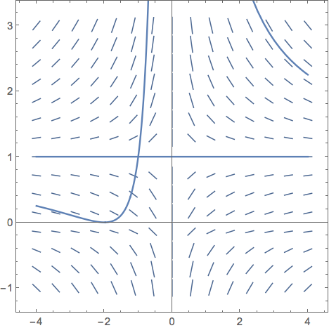
Note that the solutions intersect at the point $(-1,1)$, contradicting the existence and uniqueness theorem.

Now, in this first case, Mathematica failed to give one of the solutions, sending me an inappropriate solution, or at least it seems so to me. Now, a second case.

In[8]:= sol2 = 
 DSolve[{y'[t] == (2 Sqrt[y[t]] - 2 y[t])/t, y[-1] == 1/2}, y[t], t]

During evaluation of In[8]:= Solve::ifun: Inverse functions are being used by Solve, so some solutions may not be found; use Reduce for complete solution information. >>

During evaluation of In[8]:= Solve::ifun: Inverse functions are being used by Solve, so some solutions may not be found; use Reduce for complete solution information. >>

{{y[t] -> (Sqrt[2 (3 - 2 Sqrt[2])] + 2 t)^2/(
       4 t^2)}, {y[t] -> (Sqrt[2 (3 + 2 Sqrt[2])] + 2 t)^2/(4 t^2)}}

And the plot:

p3 = Plot[{y[t] /. sol2[[1]], y[t] /. sol2[[2]]}, {t, -4, 4}];
Show[vf, p3]

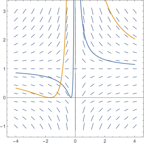
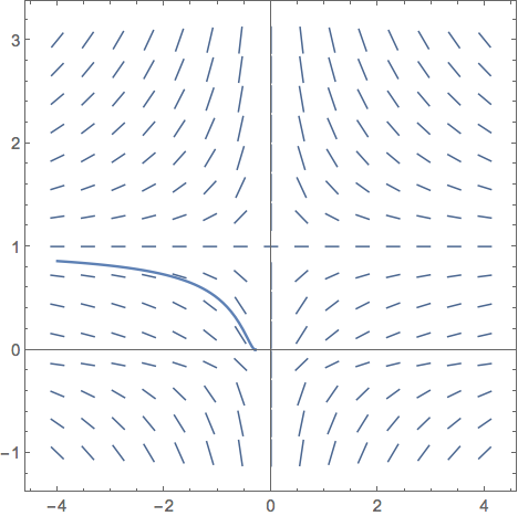
Again, two solutions intersecting at the point $(-1,1/2)$, which should not happen. What I need to know here is this: Is there an easy way in Mathematica to know which of the two selections to choose and to determine over what interval it should be plotted. Here is what I tried:

p4 = Plot[y[t] /. sol2[[1]], {t, -4, -0.292893}];
Show[vf, p4]

And the output.

But I need to learn a lot more if I am going to be helpful to my students, all of whom will be beginners in Mathematica.