This began as a light hearted attempt to simulate the rules of monopoly with the aim of maybe getting some interesting results regarding which squares are landed on the most; essentially rolling the dice N times and making a log of where the player's token ends up. And at the same time, having a means to further develop my Mathematica programming skills, as is the means by which I've learnt to use the platform so far. I naively intended this to be a weekend project where I'd maybe get a rough working model and then move on to something new. Every time I reached some milestone, I found something new to add to it, or something which I had overlooked, or something which could be done better or faster. I did some minor research on the topic while I was in the early days of this project where the best source I found was Probabilities in the Game of Monopoly®.
Ultimately, the program repeatedly takes a random integer between 2 and 12 (by default) and transforms it into an integer between 0 and 40 which form the sequence of observed player states on a Monopoly game board. Automated analysis of the resultant sequence show the empirical frequency of states, the transitional probabilities from each state and a directed graph visualising the instance of unique transitions between states.
The program has three components: the user interface and report generation, simulation of player states and analysis of data. The simulation begins by building a list of dice rolls $X$ such that $X_i$ gives the transition $n_i \rightarrow n_{i+x_i}$ for the players initial state $n_i$. Each state in the board is numbered 0 through 40 where GO is state 1, In Jail is state 0 and so on, hence representing the players position. The player is advanced according to the value of the dice while also being checked for speeding (rolling three consecutive doubles which results in immediate transition to jail). Depending on the players new state, a series of conditionals will evaluate and implement any rules which may further change the players state. When all processes are complete, the players state is appended to a list and used as the initial value for the next transition.
I - User Interface
Evaluation of the notebook upon opening returns the UI dialogue which gives the user the option to experiment beyond the games default parameters or to run the simulation as is. 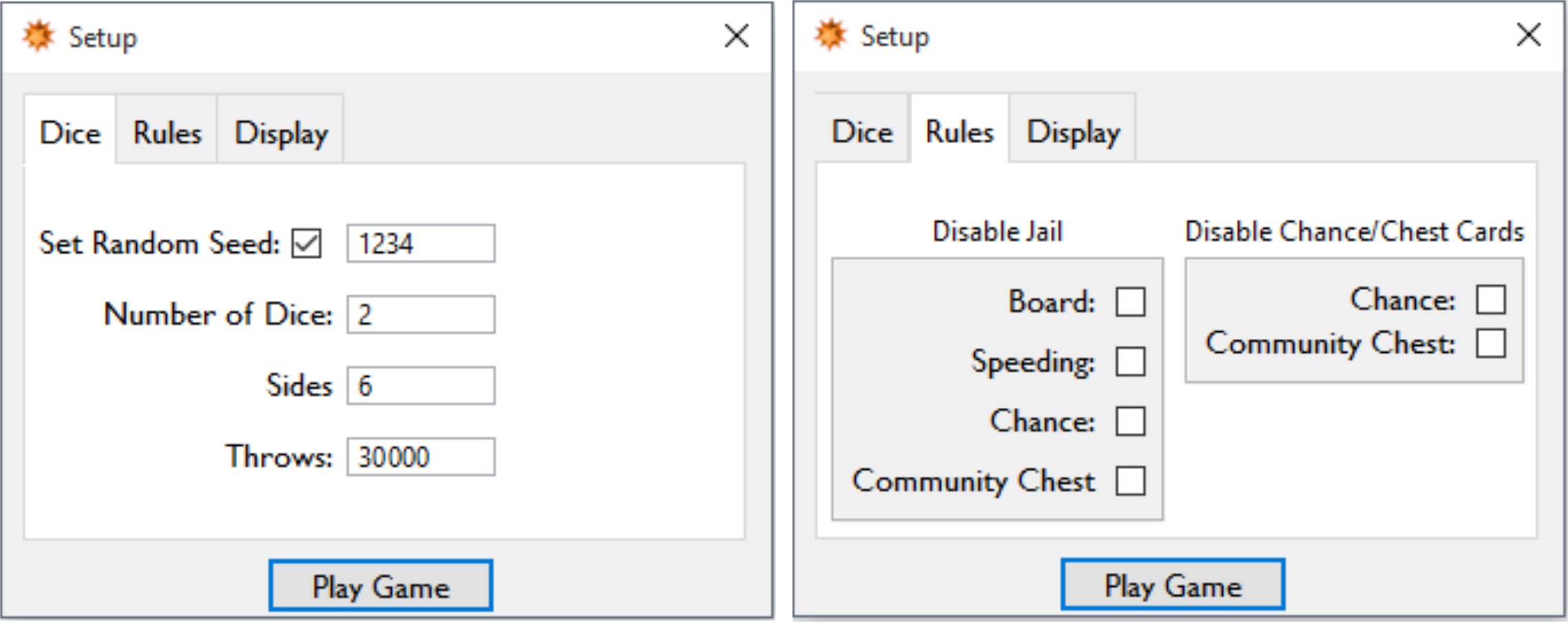
The default chain length was initially an arbitrary decision but it appears to give acceptable results without taking too long (~30 seconds on an Intel i3 laptop). In addition to allowing the user the choice of disabling elements of the analysis report, the Display tab also contains the option to choose between the UK and US localisations.
The naming conventions for each localisation are simply associations between the state index and its local name. For example:
namesUK = <|
  0 -> "In Jail", 1 -> "GO", 2 -> "Old Kent Road",...,38 -> "Park Lane", 39 -> "Super Tax", 40 -> "Mayfair", 41 -> "£"
      |>;

namesUS = <|
  0 -> "In Jail", 1 -> "GO", 2 -> "Mediterranean Avenue",...38 -> "Park Place", 39 -> "Luxury Tax", 40 -> "Boardwalk", 41 -> "$"
  |>;

names = namesUK;
where setting the value of the variable names selects the naming convention to be used.
II - Generation of Data
Clicking Play Game runs the simulation. First, it creates an array of pairs of random integers between 1 and 6 (default), establishing a list of the sum of each pair and another list which indicates if any pairs were of equal value (i.e., throwing doubles).
dice := (
   If[rndSet == 1, SeedRandom[rndSeed], SeedRandom[]];
   values = RandomInteger[{1, s}, {t, n}];
   moves = Total /@ values;
   doubles =
    Table[SameQ[values[[i, 2]], values[[i, 1]]] // Boole, {i, 1, t}]
   );
Where
In[384]:= values[[1 ;; 10]]

Out[384]= {{1, 1}, {5, 6}, {6, 3}, {1, 2}, {1, 1}, {3, 1}, {5, 3}, {3,
   1}, {6, 5}, {2, 4}}

In[386]:= doubles[[1 ;; 10]]

Out[386]= {1, 0, 0, 0, 1, 0, 0, 0, 0, 0}

In[387]:= moves[[1 ;; 10]]

Out[387]= {2, 11, 9, 3, 2, 4, 8, 4, 11, 6}
Lists and arrays storing output data are initialised and the first move is taken.
positionOld = moves[[1]] - 1;
AppendTo[transition, moves[[1]] - 1];
AppendTo[history, moves[[1]] - 1],
The list history stores the sequence of all player states while transition stores only the end points of each transition the displacement, so to speak.
The main body of the loop is now iterated for m<Length[moves].
If[positionOld == 0,
 moves[[m]] += 11],(*Adjust player starting position if leaving jail*)

If[
 doubles[[m]] == 1 && jailSpeedDisable == 0(*if player rolls doubles and jail by doubles is enabled*),
 speedingCheck++ (*Update counter*),
 speedingCheck = 0 (*Else, reset counter*)
 ],

If[
 speedingCheck == 3 (*If player has rolled three consecutive doubles*),
 positionNew = 0(*then send player to jail*);
 AppendTo[history, 0](*update position history*) ;
 speeding++(*update event tracking*),

 positionNew =
   NestWhile[# - 40 &, moves[[m]] + positionOld, # > 40 &] (*else compute the players position*);
 If[
  jailBoardDisable == 0 && positionNew == 31 (*If player's new position lands on "Go to Jail" and jail by board is enabled*),
  jail++ (*update event tracking*);
  AppendTo[history, 31 ](*update pre-jail history*);
  AppendTo[transition, positionNew];
  positionNew = 0 (*send player to jail*);
  AppendTo[history, 0] (*update position history*),

  AppendTo[history, positionNew](*Else update players new position history*)
  ]],
Since the board is 40 periodic and the players absolute position is essentially a strictly increasing sum, we need to subtract 40 from the players absolute position until a value less than 40 is returned.
NestWhile[#-40&, moves[[m]] + positionOld, #>40&]
At this point, the player has been moved and now occupies the mid turn state, the value of which is used in further conditionals to determine wherever the player should draw and implement a chance or community chest card.
chestIndex =
  {{"Advance to Go", 1},
   {"Collect " <> ToString[names[41]] <> "200", 2},
   {"Pay " <> ToString[names[41]] <> "50", 3},
   {"Collect " <> ToString[names[41]] <> "50", 4},
   ...
    {"Collect " <> ToString[names[41]] <> "10", 16},
   {"Collect " <> ToString[names[41]] <> "100 B", 17}};

chanceIndex =
  {{"Advance to Go", 1},
   {"Advance to " <> ToString[names[25]], 2},
   {"Advance to " <> ToString[names[12]], 3},
   ...
    {"Collect " <> ToString[names[41]] <> "150" , 16},
   {"Collect " <> ToString[names[41]] <> "100" , 17}};
The chance/chest card deck is a 17 by 2 array with placeholders for substitution with the designated naming convention and an index for identification. A random sample of the array is set to chest(chance)CardDeck from which the $i^{th}$ 'card' is drawn (tracked by the incremented chest(chance)CardDraw value). When the last card is drawn, the deck is re-sampled and the process is repeated.
chestCardCount++;
If[
  chestCardCount > Length[chestIndex] (*Check if deck if fully drawn*),
  chestCardDeck = RandomSample[chestIndex] (*create new reshuffled deck*);
  chestCardCount = 1 (*reset deck index*)
  ];
If the transitions to jail by a chest and or chance card are disabled and "Go to Jail" is drawn, then the program draws the next card instead or reshuffles and draws if it has reached the end of the current sample.
If[jailChestDisbale == 1 && chestCardDeck[[chestCardCount, -1]] == 6,
  Which[
   chestCardCount < 17, chestCardCount++,
   chestCardCount >= 17,
   chestCardDeck =
    RandomSample[chestIndex] (*create new reshuffled deck*);
   chestCardCount = 1 (*reset deck index*)
   ]
  ];
The $i^{th}$ card is now drawn and its identifier is set as the current chest(chance) card. cardInc is an array which tallies the events of having drawn a particular card from a certain location.
chestCard = chestCardDeck[[chestCardCount, -1]] (*takes the index of the drawn card*);
cardInc[[1, chestCard]]++;
cardInc is initialised as a constant array of zeros at the start of the simulation.
cardInc =  ConstantArray[0, {3, 17}];
(*
-- cardInc Stores incrementing values for event tracking  --,
Row 1: community chest,
Row 2: chance,
Row 3: Chance/chest position counters (chance-A,B,C, chest-A,B,C)
*)
The array cardTransition performs a task similar in scope to cardInc and is used to display mid-turn transitions from chest/chance states which aren't normally tracked otherwise. Positions 3,18 and 34 community chest states which set the value of chestLocation which relates to the relevant entry in any of the tracking arrays.
chestLocation = Which[
   positionNew == 3, 4,
   positionNew == 18, 5,
   positionNew == 34, 6
   ];
cardTransition[[chestLocation, chestCard]]++;
Rules of the drawn card are now evaluated and chestCardCount is incremented such that the next card in the current sample will drawn or re-sampled if greater than the length of the deck. Here we have that if chest card number 1 (Advance to Go) is drawn then set the players position to "GO" and update the player's position history list, if "Go to Jail" (card number 6) is drawn then send to player to jail etc.
Which[
  chestCard == 1, positionNew = 1; AppendTo[history, positionNew];  cardInc[[3, chestLocation]]++,
  chestCard == 6, positionNew = 0; AppendTo[history, positionNew];  cardInc[[3, chestLocation]]++
  ];
chestCardCount++;
Putting it all together, we get
(*  -----------  Draw a community chest  -------------  *)

If[chestCardDisable == 0,
 If[positionNew == 3(*chestA*) || positionNew == 18(*chestB*) || positionNew == 34(*chestC*),
  If[jailChestDisbale == 1 &&  chestCardDeck[[chestCardCount, -1]] == 6,
   Which[
    chestCardCount < 17, chestCardCount++,
    chestCardCount >= 17,
    chestCardDeck = RandomSample[chestIndex] (*create new reshuffled deck*);
    chestCardCount = 1 (*reset deck index*)
    ]
   ];
  chestCard = chestCardDeck[[chestCardCount, -1]] (*takes the index of the drawn card*);
  cardInc[[1, chestCard]]++;
  chestLocation = Which[
    positionNew == 3, 4,
    positionNew == 18, 5,
    positionNew == 34, 6
    ];
  cardTransition[[chestLocation, chestCard]]++;
  Which[
   chestCard == 1, positionNew = 1; AppendTo[history, positionNew];
   cardInc[[3, chestLocation]]++,
   chestCard == 6, positionNew = 0; AppendTo[history, positionNew];
   cardInc[[3, chestLocation]]++
   ];
  chestCardCount++;
  If[
   chestCardCount > Length[chestIndex](*Check if deck if fully drawn*),
   chestCardDeck = RandomSample[chestIndex](*create new reshuffled deck*);
   chestCardCount = 1(*reset deck index*)
   ];
  ]
 ],
The routine for drawing a chance card follows the same procedure but is longer since most of the deck contains cards which will invoke some mid-turn transition.
The player's turn in now over and the new position is set as the old position and transition is now updated such that it only sees the players end of turn state.
AppendTo[transition, positionNew],
positionOld = positionNew
III - Analysis of Data: Player States
Lets examine the raw data.
In[433]:= history[[1 ;; 10]]

Out[433]= {1, 3, 0, 22, 31, 0, 14, 16, 20, 28}

In[434]:= history[[1 ;; 10]] /. names

Out[434]= {"GO", "Community Chest A", "In Jail", "Strand", "Go To Jail", "In Jail", "Whitehall", "Marylebone Station", "Vine Street", "Coventry Street"}

In[438]:= transition[[1 ;; 10]] /. names

Out[438]= {"GO", "In Jail", "Strand", "Go To Jail", "In Jail", "Whitehall", "Marylebone Station", "Vine Street", "Coventry Street", "Regent Street"}
This tells us that the players first turn originated at "GO", landed on and drew a community chest card and was sent to jail. Hence, the first transition is $0 \rightarrow 1$ or $\text{GO}\rightarrow\text{In Jail}$ or $\text{GO}\rightarrow\text{Community Chest A}\rightarrow\text{In Jail}$, depending on how you you want to perceive it. We'll be doing it both ways for the analysis.
Since it is not possible (by default) to end ones turn on "Go to Jail" (as it instantly advances the player to a different state) and likewise with certain instances of chance and community chest cards, a chart of end of turn states would under represent the instances of these such positions. Fortunately, all mid-turn transition events are tracked separately so a new array of player states with entries for end and mid turn observations can be easily made.
position =
  MapAt[(*chestC*)# - cardInc[[3, 6]] &, {35, 3}][
   MapAt[(*chestB*)# - cardInc[[3, 5]] &, {19, 3}][
    MapAt[(*chestA*)# - cardInc[[3, 4]] &, {4, 3}][
     MapAt[(*chanceC*)# - cardInc[[3, 3]] &, {38, 3}][
      MapAt[(*chanceB*)# - cardInc[[3, 2]] &, {24, 3}][
       MapAt[(*chanceA*)# - cardInc[[3, 1]] &, {9, 3}][
        ReplacePart[
           {
           (*Chance Advancements*)
           {9, 4} -> cardInc[[3, 1]],
           {24, 4} -> cardInc[[3, 2]],
           {38, 4} -> cardInc[[3, 3]],
           (*Community Chest Advancements*)
           {4, 4} -> cardInc[[3, 4]],
           {19, 4} -> cardInc[[3, 5]],
           {35, 4} -> cardInc[[3, 6]],
           (*Go To Jail*)
           {32, 3} -> If[jailBoardDisable == 0, 0, testData[[32, 2]]],
           {32, 4} -> If[jailBoardDisable == 0, jail, 0]
           }
          ][Thread[{
             First /@ #,
              StringPadRight[#, Max[StringLength[#]],"."] &[(First /@ # /. names) &[testData]],
             Last /@ #,
             0
             }] &[testData]
         ]
        ]
       ]
      ]
     ]
    ]
   ];
This outputs the array
{{0, "In Jail.................", 2, 0}, {1, "GO......................", 5, 0}, {2, "Old Kent Road...........", 3, 0}, {3, "Community Chest A.......", 2, 1},...}
which has general form of $\{\{n_i,\text{"name"},\text{end turn observed},\text{mid turn observed}\},...\}$
For example, position[[4]] returns data for "Community Chest A" (the first chest state) which is the fourth possible state (counting from "Jail"),
{3, "Community Chest A.......", 2, 1}
This means that the player occupied "Community Chest A" three times in total, but was advanced mid turn once (via drawing "Go to Jail"), hence ended the turn in the same state only twice. This was calculated by subtracting the number of times the player was advanced from "Community Chest A"(cardInc[[3, 4]]) from the number of times the player was observed in the state "Community Chest A" (position[[4,3]]). The value cardInc[[3, 4]] then replaces position[[4,4]] which is 0 by default.
Yet, we're still not ready to show the results since were using observables; if a state was never occupied (inevitable for results using small chain lengths or disabled Jail) it will not be present in the results, yet the chart of observed states expects a list of all 41 states - even the null cases. Thus, we need to identify if any are missing and insert them into the list which position is generated from.
    testData = SortBy[Tally[history], First];
    target = Range[0, 40];
    Label[start]; If[Length[testData] != Length[target],
     testData =
      Quiet[(Insert[{Evaluate[Min[Flatten[ Position[Table[(First /@ testData)[[i]] === target[[i]], {i, 1, 41}], False]]] - 1], 0},
          Min[Flatten[Position[Table[(First /@ testData)[[i]] === target[[i]], {i, 1, 41}], False]]]]@testData)]];
    If[Length[testData] != Length[target],Goto[start]];
It was originally a quick fix implementation to test the solution (inspired by an other program of similar scope I hastily wrote a couple months back) - but it works!
In[524]:= SortBy[Tally[history], First]

Out[524]= {{0, 1}, {1, 3}, {3, 1}, {4, 1}, {6, 1}, {8, 1}, {10,1}, {14, 2}, {15, 1}, {17, 1}, {23, 2}, {24, 2}, {26, 1}, {27,1}, {29, 1}, {30, 1}, {31, 1}, {34, 1}, {38, 1}}

In[528]:= testData

Out[528]= {{0, 1}, {1, 3}, {2, 0}, {3, 1}, {4, 1}, {5, 0}, {6, 1}, {7,0}, {8, 1}, {9, 0}, {10, 1}, {11, 0}, {12, 0}, {13, 0}, {14, 2}, {15, 1}, {16, 0}, {17, 1},{18, 0}, {19, 0}, {20, 0}, {21,0}, {22, 0}, {23, 2}, {24, 2}, {25, 0}, {26, 1}, {27, 1}, {28,0}, {29, 1}, {30, 1}, {31, 1}, {32, 0}, {33, 0}, {34, 1}, {35,0}, {36, 0}, {37, 0}, {38, 1}, {39, 0}, {40, 0}}
The position array can now be presented in table form
$ \begin{array}{cccc} 0 & \text{In Jail.................} & 1151 & 0 \ 1 & \text{GO......................} & 950 & 0 \ 2 & \text{Old Kent Road...........} & 623 & 0 \ 3 & \text{Community Chest A.......} & 609 & 70 \ 4 & \text{Whitechapel Road........} & 661 & 0 \ 5 & \text{Income Tax..............} & 718 & 0 \ 6 & \text{King's Cross Station....} & 855 & 0 \ 7 & \text{The Angel Islington.....} & 653 & 0 \ &.&&\ &.&&\ &.&&\ 37 & \text{Chance C................} & 322 & 379 \ 38 & \text{Park Lane...............} & 659 & 0 \ 39 & \text{Super Tax...............} & 644 & 0 \ 40 & \text{Mayfair.................} & 646 & 0 \ \end{array} $
and plotted as a stacked bar chart
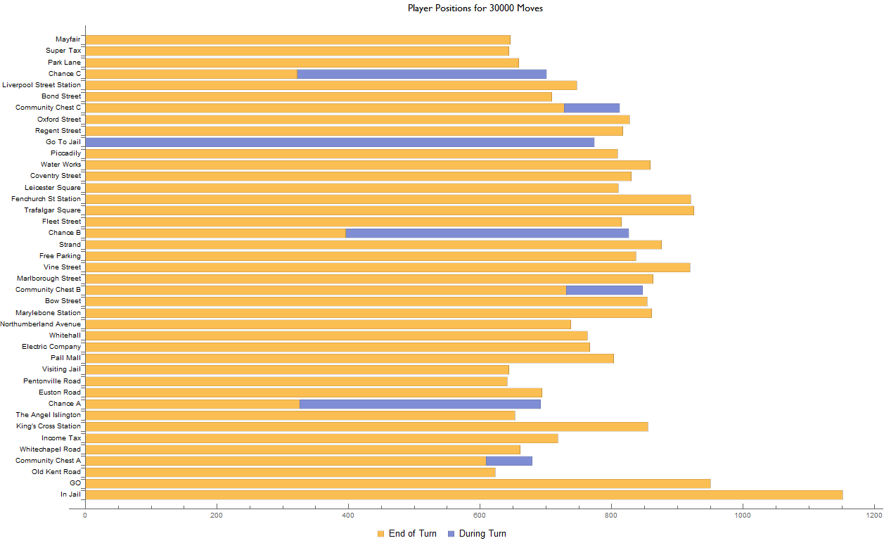
Since about 60% of the chance card deck will invoke a mid-turn transition, we can expect similar proportions when examining the ratio between the end and mid turn results for any of the "Chance" states, which is on average 53% for this dataset. The same reasoning also holds for the community chest states, of which 12% of the deck will advance the player and "Go to Jail" which by default will always advance the player mid turn.
Of the many vectors which sink the player into jail (rolling three consecutive doubles, "Go to Jail" and chance & community chest cards, which we'll visualise soon) combined with the expected outcome of rolling two 6-sided fair dice, the distribution of player states experiences a peak around 7 states after "In Jail". Furthermore, states which are three spaces prior to any chance card state see a slightly higher incidence rate as when compared to their neighbours; this may be attributed to the "Go Back Three Spaces" card present in the chance deck. The same can be said for states which are the subject of dedicated advance cards in the chance/chest card deck i.e., "Advance to Go", "Advance to Trafalgar Square", etc.
The multiple mid-turn advancement rules are what makes Monopoly such an interesting system and does well to balance the game in subtle ways. For instance, many players will strategize to acquire the orange properties during the mid-game stage, justifiable in part due to the 7 After Jail Peak.
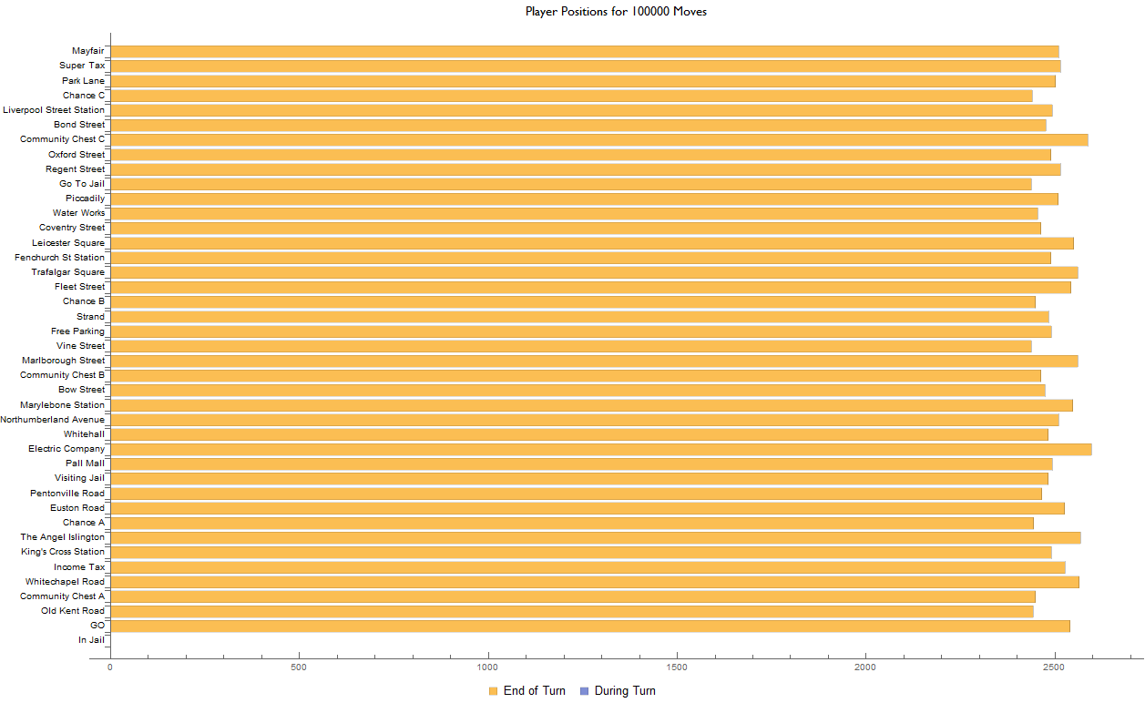
Running the simulation again under the same random seed but for a chain length of 100 000 moves and with all advancement rules disabled, one can immediately see how boring the game would be otherwise (or even more boring if you're so inclined!).
III - Analysis of Data: Player Transitions
We've seen the distribution of states - the cause. But what about the effect - or rather the transitions to states?
Since the end of turn transitions are tracked individually, visualising them is (almost) very easy.
We begin by arranging the transition list into an N by 2 array
transChart = Join[trans, Table[{transition[[i]], transition[[i + 1]]}, {i, 1, Length[transition] - 1}]];

  In[752]:= transChart[[1]]

Out[752]= {8, 1}
This reads as $\{\{8\rightarrow1\},...\}$
The next function tallies the transitions, extracts all entries originating from a given state and sorts them by the number of times they were observed. Since the transitional origin needs prior specification, it is now unnecessary and is dropped from the result.
transitionExtract = SortBy[Rest /@ ArrayReshape[#, {Length[#], 3}], First] & [Tally[Extract[transChart, Position[transChart, {#, _}]]]] &;

In[750]:= transitionExtract[1]

Out[750]= {{0, 17}, {1, 12}, {3, 27}, {4, 55}, {5, 91}, {6, 114}, {7,142}, {8, 66}, {9, 137}, {10, 90}, {11, 68}, {12, 68}, {13,34}, {16, 22}, {25, 7}}
This means that, starting from state 1, the player ended on state-7 142 times, i.e., $(1\rightarrow7)$ was observed 142 times.
The counts of each extracted transition are now normalized and presented as percentage probabilities
transitionProb = Thread[{First /@ transitionExtract[#], N[Last /@ transitionExtract[#]/Total[Last /@ transitionExtract[#]]*100, 2]}] &;

In[751]:= transitionProb[1]

Out[751]= {{0, 1.8}, {1, 1.3}, {3, 2.8}, {4, 5.8}, {5, 9.6}, {6,12.}, {7, 15.}, {8, 6.9}, {9, 14.}, {10, 9.5}, {11, 7.2}, {12, 7.2}, {13, 3.6}, {16, 2.3}, {25, 0.74}}
So, for the set of transitions $(1\rightarrow{n_i})$, $P(i=7)=0.15$ and so on...
We generate a bar chart and use the dynamic variable z to select the argument for the function transitionProb. This is controlled via a popup menu.
Dynamic[
 BarChart[
    Apply[Labeled,
     Reverse[Thread[{First /@ # /. names, Last /@ #}] &[transitionProb[#]], 2], {1}],
    BarOrigin -> Left,
    PlotLabel -> Row[{
       menuStyle["End of Turn Transition Probabilities (%) From ", ""],
       Spacer[5],
       PopupMenu[Dynamic[z], Table[i -> names[i], {i, 0, 40}]]
       }],
    ImageSize -> {resX/3}
    ] &[z]]
Lets see what it looks like!
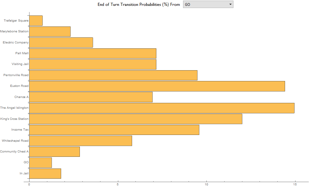
Normally, the mid turn transitions caused by chance/chest would not be visible when viewing those particular states so they are added in manually within the transChart function in the form of the array trans
Notice the proportion of "Chance A" with respect to it's neighbours; the transition $(1\rightarrow8)$ requires the condition that one did not draw an advancing chance card. The alternative - that one did draw and advancing chance card - explains why states normally out of the dices default range (Trafalgar Square, for instance) are also valid transitions. Lastly, if we consider the case of having rolled 2 consecutive doubles prior to any current state, there is a chance that the player will be sent to jail, thus "In Jail" will (by default) be adjacent to any other state (in addition to the trivial case of "Go to Jail"). The simulation does not implement any rules regarding leaving jail and so the player leaves jail as it would with any other state.
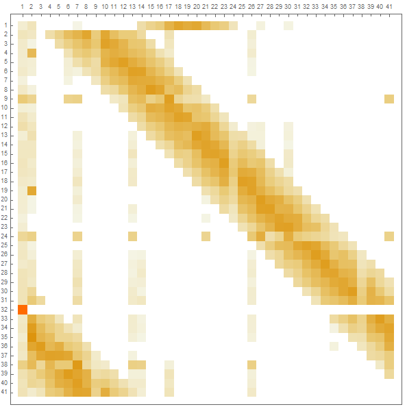
While on the topic of adjacency, we can take each object returned by transitionProb for values 0 through 40 and build a transition matrix. We'll need to also pad each row with it's null values, like we did when generating the position array.
(*
transMatrix:

               j1=jail   j2=Go  . . .
  i1=jail    i -> j
  i2=Go
  .
  .
  .

i->j=transMatrix[[i,j]] for i,j = 1,2,3...41
*)

j = 0; target = Range[0, 40]; transMatrix = {}; fill = Thread[{First /@ #, Last /@ #}] &[transitionProb[j]]; Label[start]; If[Length[fill] != Length[target],
 fill = Quiet[(Insert[{Evaluate[Min[Flatten[Position[Table[(First /@ fill)[[i]] === target[[i]], {i, 1, 41}],  False]]] - 1], 0},
      Min[Flatten[Position[Table[(First /@ fill)[[i]] === target[[i]], {i, 1, 41}], False]]]]@fill)]];
 If[Length[fill] != Length[target], Goto[start], AppendTo[transMatrix, Last /@ fill];
   j++;
    If[j <= 40, fill = Thread[{First /@ #, Last /@ #}] &[transitionProb[j]];
     Goto[start]]];
The resultant transition matrix may be viewed as a table
TableForm[transMatrix,
 TableHeadings -> {StringPadLeft[Most[Values[names]], Max[StringLength[Most[Values[names]]]], " "], Table[Rotate[Most[Values[names]][[i]], [Pi]/2], {i, 1, 41}]},
 TableAlignments -> {Left, Bottom}]
or visualised more compactly via a matrix plot which shows rates of adjacency between states. For reference, "In Jail " is state 1 and "Go to Jail" is state 32, such that $P(1|32)=1.0$.
adjacencyMatrix = MatrixPlot[transMatrix,FrameTicks -> {{Range[41], None}, {None, Range[41]}}]
III - Analysis of Data: Visualizing Transitions
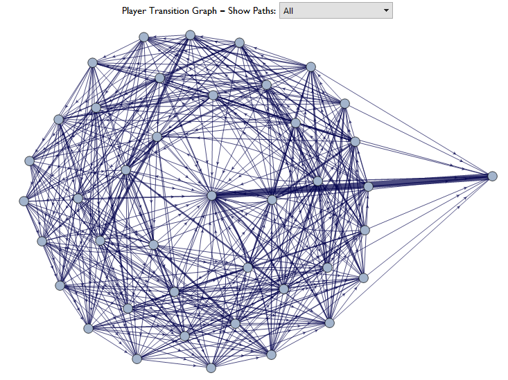
I wanted to save the best for last. Although the transition graph isn't as explicit as the charts, it looks cool and is fun to play with so it satisfies the projects original desire.
I quickly learnt that I could not just simply make a table of directed edges using history and call it a day; such a graph was saturated with edges and essentially useless.
First, we do indeed make a table of all directed edges.
a = Table[(First /@ trans)[[i]] \[DirectedEdge] (Last /@ trans)[[i]], {i, 1, Length[trans]}];
b = Table[history[[i]] \[DirectedEdge] history[[i + 1]], {i, 1, Length[moves] - 1}];
net = Join[a, b];
But then it is tallied so that each transition is represented only once.
data = First /@ SortBy[Tally@net, Last] /. names;

tally = N[Normalize[Last /@ SortBy[Tally@net, Last]]]/30;
The list data is a sample of each transition as a directed edge where the $i^{th}$ entry of tally corresponds to the $i^{th}$ entry of data and is proportionate to the number of times its respective transition was observed.
In[808]:= data[[1 ;; 5]]

Out[808]= {"In Jail" -> "In Jail", "Pall Mall" -> "In Jail", "Electric Company" -> "In Jail", "Whitehall" -> "In Jail", "Liverpool Street Station"->"In Jail"}

In[809]:= tally[[1 ;; 5]]

Out[809]= {0.000018484, 0.000018484, 0.000018484, 0.000018484, 0.000018484}
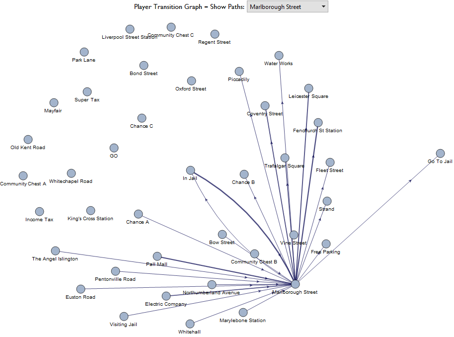
We'll use this data to modify the edge style, thus representing the occurrence of each transition in terms of its edge thickness. And like the transition probability chart, a popup menu allows the user to view specific points of origin.
view = "null"(*Set default*);
colour = RGBColor[0, 0, 0.3];

Dynamic[

 a = Table[(First /@ trans)[[i]] \[DirectedEdge] (Last /@ trans)[[
     i]], {i, 1, Length[trans]}];
 b = Table[
   history[[i]] \[DirectedEdge] history[[i + 1]], {i, 1,
    Length[moves] - 1}];
 net = Join[a, b];
 data = First /@ SortBy[Tally@net, Last] /. names;
 tally = N[Normalize[Last /@ SortBy[Tally@net, Last]]]/30;
 graph = Graph[data];
 contains = colour;
 If[view != "null",
  contains = Total /@ (Partition[StringContainsQ[Flatten@Thread[{First /@ EdgeList[graph], Last /@ EdgeList[graph]}], ToString[view /. names]],2]//Boole) /. {1 -> colour, 0 -> Opacity[0]}];

 Graph[data,
  VertexLabels -> If[graphLabel == 1, Placed[{"Name"}, Tooltip], Placed["Name", Above]],
  EdgeShapeFunction -> GraphElementData[{"ShortFilledArrow", "ArrowSize" -> .01}],
  EdgeStyle ->  Apply[Rule, Thread[{EdgeList[graph], Thread[{Thickness /@ tally, contains}]}], {1}],
  ImageSize -> Scaled[0.55],
  PlotLabel -> Row[{menuStyle["Player Transition Graph - Show Paths: ", ""],
     PopupMenu[Dynamic@view, Insert[Table[i -> names[i], {i, 0, 40}], "null" -> "All", 1]]}]
  ]]
The vertex labels have been deployed as tool-tips by default but the option for standard labelling also exists.
Here we can see again that jail is a significant source when examining Marlborough Street.
Lets run the simulation again but play the game where only doubles are thrown (I made an ad hoc moves list for this since its an idea I just thought of now). We'll also disable jail by speeding - this could be done in real life in the form of a house rule.
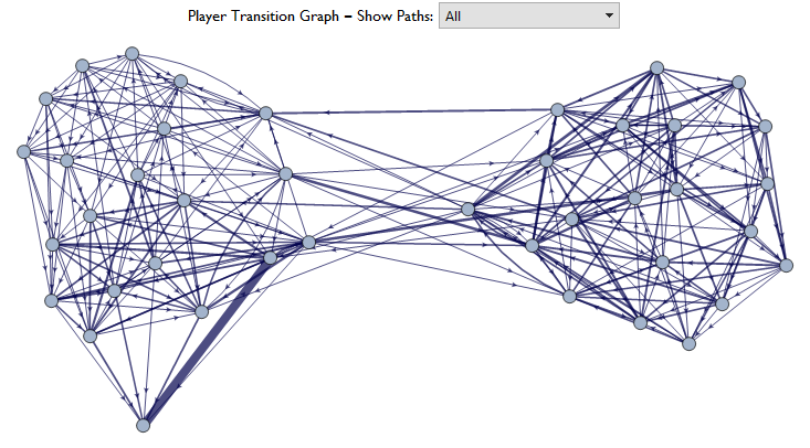
Highlighting the graphs Hamiltonian Cycle shows that its possible to win Monopoly in a single turn sustained by rolling doubles since one can buy up all the properties, provided that you agree to the modified rules.
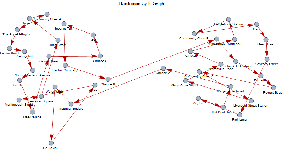
If we extract the Hamiltonian transitions and cross reference them with the probability transition matrix, we can see how likely such an event would be.
In[261]:=
hData = ((RotateRight[Flatten[#2], #]) &[(Length[Flatten[#]] - Position[#, 1 \[DirectedEdge] _, 2][[1, 2]] + 1) &[#], #]) &[
   FindHamiltonianCycle[Graph[First /@ SortBy[Tally@net, Last]]]];

hTransitionProbabilities = Table[transMatrix[[#2[[#, 1]], #2[[#, 2]]]] &[i, Thread[{First /@ hData, Last /@ hData}] + 1], {i, 41}]/100

Times @@ hTransitionProbabilities


Out[262]= {0.13, 0.14, 0.071, 0.058, 0.14, 0.18, 0.16, 0.17, 0.13, 0.21, 0.19, 0.16, 0.16, 0.19, 0.15, 0.14, 0.18, 0.15, 0.16, 0.18, 0.19, 0.14, 0.10, 0.064, 0.17, 0.17, 1.0, 0.17, 0.18, 0.16, 0.16, 0.19, 0.13, 0.15, 0.20, 0.17, 0.15, 0.14, 0.23, 0.068, 0.14}

Out[263]= 0.*10^-34
$P(H)\approx10^{-34}$, so not likely.
Please have fun experimenting with the program and informing me of any errors in my analysis. I'm planning on returning to it at some point in the near future, either by repeating the analysis using a theoretical Markov transition matrix and using these empirical results as a benchmark or simulating a two player game and seeing what happens. In the mean time, I have a project from August which I want to revisit.
Regards,
Ben
 Attachments:


