Hi Doug, I see you have a lot of scatter in the red, just like me. Maybe it's inherently hard to discern the square. I was looking through the demonstrations and came across a demo of a disk of random dots moving in a field of random dots. As soon as you stopped moving the disk, it just settled into the background and became invisible. Maybe if the inner square were moving, it would be easier to see. Something to try. Here is a new, much easier version. I found out how to detect MouseUp events by using TrackingFunction[]. Now all you have to do is detect the inner square and release the mouse button. The three buttons have been turned into Reset buttons. If you aren't happy with one of the graphs, you can delete it and re-do it. 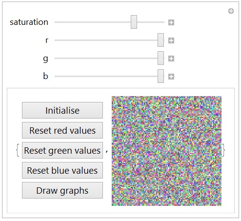
A notebook is attached. Eric
 Attachments:
|
|
|
Eric, Here are two more trials. I have a hardcover copy of Ishihara, and I pass. Doug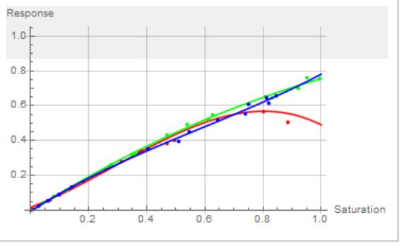 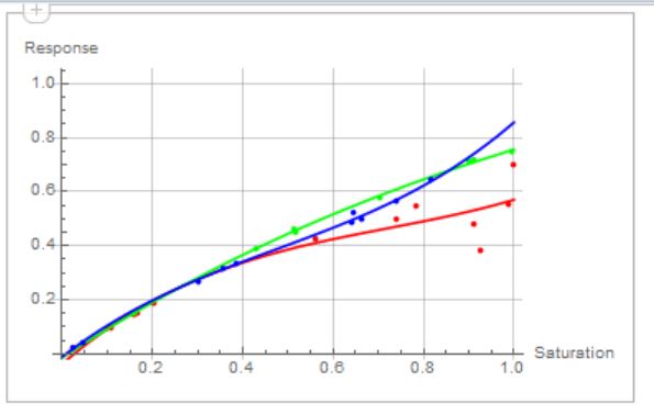
|
|
|
Hi Doug, Are we seeing the effect of the yellowing of your lenses in the waviness of your blue and green lines? I should add in my instructions that it's important to go close to the very ends of the saturation, otherwise the curves extrapolate in weird ways. Are you normally aware of a red deficiency? Eric
|
|
|
Hello everyone, Here is a functional app to measure colour blindness. 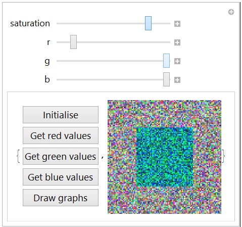
Instructions 1) Click on Initialise to set the data collection arrays to zero. 2) A random saturation level for the image will be selected. Move one of the r, g, or b sliders until the central square appears. Keep adjusting the slider until the square is just visible. Click on the corresponding Get colour values button. 3) A new random saturation will appear. Continue until you have enough data points to generate smooth graphs. 4) Click on Draw graphs. A new notebook will appear with the graphs, data arrays, and the approximating equation. 5) Examine the graphs for regions that need more data. Go back to the tester and manually set the Saturation slider to the value needed. This can be done by positioning the slider visually so that it is matches the horizontal axis of the region needing data. Discussion This app is an implementation of a technique due to Douglas Youvan. There is a significant improvement that eludes me, so I'm asking for help. It isn't necessary to click on the Get colour values button. All that is required is to sense the mouse up when the slider is released. Suggestions? I know that EventHandler[] is probably the way to go, but how do you relate the MouseUp to a particular slider? It would be interesting to get some graphs from both normal and colour blind people. There are other types of colour blindness than red/green. (I always thought that my green vision must be defective, too. Not so.) And suggestions for improvements and other features would be welcome. A notebook is attached. Eric
Attachments:
|
|
|
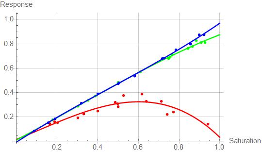
Eric, I took the test twice. The values were very similar, and my red consistently fell off as shown in the attached gif. Doug
Attachments:
|
|
|
Hi Doug, Here is the result with my amber-tinted sunglasses:
 And that's why the fall colours explode with them on! Eric
|
|
|
Eric, Phenomenal! This belongs in a vision book that can display your work. You are on a roll, so I don't want to divert you. But, could I suggest that you try "ortho" on an image that is invisible because of your deficit? Although I pass Ishihara, Ortho should pick up images that I can't see either. Also, I have yet to find any "Daltonization" algorithms. Doug
|
|
|
Hi Doug, I fixed the code to make collecting data easier:
valsb = {};

Manipulate[{Button["Get values",
   AppendTo[
    valsb, {1 - saturation - offset,
     b (1 - saturation - offset)}]], (image =
    ImageData[
     RandomImage[{saturation + offset, 1.0}, {100, 100},
      ColorSpace -> "RGB"]];
   ImageCompose[Image[image, ImageSize -> 200],
    Image[Partition[
      Transpose[{r, g, b}*
        Transpose[Flatten[image[[25 ;; 75, 25 ;; 75, All]], 1]]], 50],
      ImageSize -> 200]])}, {{offset, 0}, .05, -.05}, {{saturation,
   0.5}, .95, 0.05}, {{r, 1.0}, 0.0, 1.0}, {{g, 1.0}, .85,
  1.0}, {{b, 1.0}, .85, 1.0}]
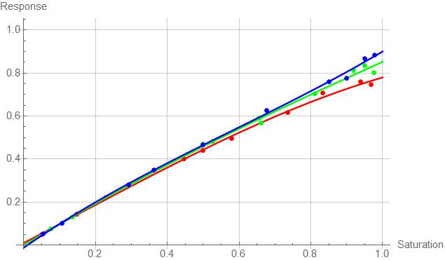
The AppendTo[] function adds the data points directly to the list, which is valsb for the blue. More work on the interface is needed for an operational app, of course. Using a different monitor, I got these results: 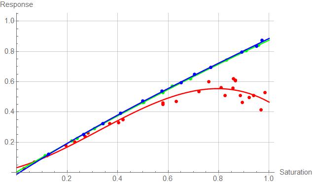
Maybe I'm just getting better at taking the test. In both cases, though, the red scatter is appreciable. Now I know why I can't pick raspberries! Eric
|
|
|
Hi Doug, I've been testing myself. Here is the new code:
Manipulate[
  {
     PasteButton["Get values",{1-saturation-offset, b(1-saturation-offset)}],
     (image=ImageData[RandomImage[{saturation+offset,1.0},{100,100},ColorSpace->"RGB"]];
     ImageCompose[Image[image,ImageSize->200],
     Image[Partition[Transpose[{r,g,b}*Transpose[Flatten[image[[25;;75,25;;75,All]],1]]],50],ImageSize->200]])
  },
  {{offset,0},.05,-.05},{{saturation,0.5},.95,0.05},{{r,1.0},0.0,1.0},{{g,1.0},.85,1.0},{{b,1.0},.85,1.0}
]
To make the sliders less sensitive, I added a finer Saturation control. This isn't strictly necessary, because pressing the alt key while moving the sliders increases their sensitivity by 10. But that's an esoteric feature some might not know. The response is taken as the red slider, say, multiplied by the saturation being tested. In the cases of the green and blue, this makes the response almost equal to the stimulus. But for the red, things are very different. There is also a PasteButton[], which sends the values of the test datum to the current output position in the notebook. These form a series of lists, but commas and surrounding braces need to be added to finish them off. The values are fitted to a third order polynomial. Here the blue values are fitted:
xxxb=Fit[valsb,{1,x,x^2,x^3},x]
The whole set of data points and fitted functions look like this:
Show[
   ListPlot[valsr, PlotStyle -> Red],
   Plot[eqnr[x], {x, 0, 1}, PlotStyle -> Red],
   Plot[eqng[x], {x, 0, 1}, PlotStyle -> Green],
   ListPlot[valsg, PlotStyle -> Green],
   ListPlot[valsb, PlotStyle -> Blue],
   Plot[eqnb[x], {x, 0, 1}, PlotStyle -> Blue],
   PlotRange -> {{0, 1}, {0, 1}}, AxesOrigin -> {0, 0},
   AxesLabel -> {Saturation, Response}
]
Eric
|
|
|
Hey Eric, Before I comment on your recent work, let me upload another program here. This started at: http://et-al.com/pdf/document3.pdf . Look at Figure 5, panel F and the math that goes with it. I re-wrote that code in Examples 3 and 4 in my Pseudocolor e-book in 2006: http://youvan.com/Examples/Example_4._Counterfeit_Detection_Based_on_Ink_Color.htm . Here, I've attached "otho 1" which is running in version 10.3. The main thing to note in the code is that on images with homogenous backgrounds the matrix will get identical pixel values and blow up from singularity. That's why you see me adding small random numbers. I've now uploaded "ortho 2 click", and it is much easier to use. You get to pick three pixels (colors) and then orthonormalize the entire image. Doug
Attachments:
|
|
|
Hey Eric, Before I comment on your recent work, let me upload another program here. This started at: http://et-al.com/pdf/document3.pdf . Look at Figure 5, panel F and the math that goes with it. I re-wrote that code in Examples 3 and 4 in my Pseudocolor e-book in 2006: http://youvan.com/Examples/Example_4._Counterfeit_Detection_Based_on_Ink_Color.htm . Here, I've attached "otho 1" which is running in version 10.3. The main thing to note in the code is that on images with homogenous backgrounds the matrix will get identical pixel values and blow up from singularity. That's why you see me adding small random numbers. Ortho 1 picks points randomly, but it is also advantageous to let the user do three mouse clicks for red, green, and blue. Those colors will be remapped to full color R, G, and B and every other color in between will be warped into these new color axes. Eric - The second figure here: http://www.vischeck.com/daltonize/ is startling if it is correct. The deficit would seem to rule-out work in fluorescence microscopy. We also see reference in this link to "Daltonization". I'll look for the algorithms, next. Could you please send a "hello" to doug@youvan.com ? More soon ... Doug
Attachments:
|
|
|
Hi Doug, Have you come up with anything? This morning I discovered RandomImage[], and in true MMA style, it's very fast. Instead of a cross in the square, I used a square inside a square. I also found an interesting thing about the saturation (correct term?) of the background image. When it is at full saturation, I can only barely see the interior square when r is at zero. Here's the code:
        Manipulate[
           (
              imag=ImageData[RandomImage[{saturation,1.0},{100,100},ColorSpace->"RGB"]];
              ImageCompose[Image[imag,ImageSize->200],
              Image[Partition[Transpose[{r,g,b}*Transpose[Flatten[imag[[25;;75,25;;75,All]],1]]],51],ImageSize->200]]
            ),
            {{saturation,0.5},1,0},{{r,1.0},0.0,1.0},{{g,1.0},0.0,1.0},{{b,1.0},0.0,1.0}
        ]
The reason I can see the green and blue so well is that I have lens implants in both eyes. The ophthalmologist showed me a yellow glass lens that he keeps in his office to show his patients how discoloured the lens becomes with age. It took a few months to get over the extreme blueness of my new vision. But I also remembered how blue snow used to look when I was a child. Eric
Attachments:
|
|
|
Hi Doug, The number of calculations for a single frame is 60,000 + the cross. To get the sort of scintillation you want, it looks like the background should be pre-calculated. Here is a first attempt that you can play with.
r=.5;b=1;g=1;
col=Table[For[i=1,i<=100,i++,For[j=1,j<=100,j++,tab2[[i,j]]={RandomReal[{RandomReal[],1.0}],RandomReal[{RandomReal[],1.0}],RandomReal[{RandomReal[],1.0}]}]]

For[i=47,i<=53,i++,For[j=1,j<=100,j++,tab2[[i,j]]={RandomReal[{RandomReal[],r}],RandomReal[{RandomReal[],g}],RandomReal[{RandomReal[],b}]}]]

For[i=1,i<=100,i++,For[j=47,j<=53,j++,tab2[[i,j]]={RandomReal[{RandomReal[],r}],RandomReal[{RandomReal[],g}],RandomReal[{RandomReal[],b}]}]]

Image[tab2,ImageSize->{400,400}],30];
This creates a list of 30 backgrounds plus the cross set by the rgb values at the start. I can see the cross at higher values of red when the display is animated. Here is the animation.
ListAnimate[col, 16]
Next is to put this into a Manipulate. Tomorrow. Eric
|
|
|
Erik, I've now played with the test. You are better than me with G and B. However, R=0.4 is vivid Cyan to me. The longer I look at the figure, the less confident I am. Can you make the figure regenerate even when the sliders are not moving? That would eliminate bad random numbers and give more of an average for that value. Also, it might eliminate this saturation effect by distracting you with new images. Doug
|
|
|
Eric, I am still playing with your very nice code. Last night, I did about the same thing with a plethora of cut and paste jobs! By Ishihara, I am not color blind. Your code would be appreciated as CDF. There are other people interested that do not have Mathematica. I'll get you some thresholds for my own vision. There's another color blind guy who has been looking at my work, but he would need a CDF. I'm thinking we need to do something like balance these in Monochrome, so there is no hint of intensity. Beware of ColorConvert to grayscale - it does not do what you would expect on conversion to grayscale. (It's not a simple average). More later ... Doug
|
|
|
Hi Doug, I played around with the colour blind test here: Ishihara. I can't see anything, even the one that red/green colour blinds are supposed to see. My wife could see everything. Then I tried Color Arrangement Test and was rated as severely colour blind. So I tried it with my sunglasses on and was told I am not colour blind at all! Back to the Ishihara test with the sunglasses and I still couldn't see anything. So the sunglasses do provide some correction. Here is your code with a manipulate for the red, green, and blue components.
tab1 = Table[{x, y}, {x, 100}, {y, 100}];
tab2 = tab1;
cbTest[r_, g_, b_] :=
  (For[i = 1, i <= 100, i++,
    For[j = 1, j <= 100, j++,
     tab2[[i, j]] = {RandomReal[{RandomReal[], 1.0}],
       RandomReal[{RandomReal[], 1.0}],
       RandomReal[{RandomReal[], 1.0}]}]]

   For[i = 47, i <= 53, i++,
    For[j = 1, j <= 100, j++,
     tab2[[i, j]] = {RandomReal[{RandomReal[], r}],
       RandomReal[{RandomReal[], g}], RandomReal[{RandomReal[], b}]}]]

   For[i = 1, i <= 100, i++,
    For[j = 47, j <= 53, j++,
     tab2[[i, j]] = {RandomReal[{RandomReal[], r}],
       RandomReal[{RandomReal[], g}], RandomReal[{RandomReal[], b}]}]]

   Image[tab2, ImageSize -> {400, 400}])

Manipulate[cbTest[r, g, b],
    {{r, 1.0}, 0.0, 1.0}, {{g, 1.0}, 0.0, 1.0}, {{b, 1.0}, 0.0, 1.0}]
I can start to see the cross with red at 0.4 and the others at 1.0,
but with my sunglasses on, 0.74 I can start to see the cross with green at 0.875 and the others at 1.0. I can start to see the cross with blue at 0.833 and the others at 1.0. Are you colour blind? If so, what values do you get? See attached notebook for code. Eric
Attachments:
|
|
|
Eric, How is this for a start? Doug
tab1 = Table[{x, y}, {x, 100}, {y, 100}];
tab2 = tab1;
For[i = 1, i <= 100, i++, For[j = 1, j <= 100, j++, tab2[[i, j]] = {
    RandomReal[{RandomReal[], 1.0}],
    RandomReal[{RandomReal[], 1.0}],
    RandomReal[{RandomReal[], 1.0}]} ]]

For[i = 47, i <= 53, i++, For[j = 1, j <= 100, j++, tab2[[i, j]] = {
    RandomReal[{RandomReal[], 0.5}],
    RandomReal[{RandomReal[], 1.0}],
    RandomReal[{RandomReal[], 1.0}]} ]]

For[i = 1, i <= 100, i++, For[j = 47, j <= 53, j++, tab2[[i, j]] = {
    RandomReal[{RandomReal[], 0.5}],
    RandomReal[{RandomReal[], 1.0}],
    RandomReal[{RandomReal[], 1.0}]} ]]

Image[tab2, ImageSize -> {500, 500}]
|
|
|
Hi Douglas, The fall colours have finished in Nova Scotia. Viewed directly, there isn't anything very spectacular, but when I put on my amber-tinted sunglasses, the reds become vibrant. So the sunglasses seem to give me normal colour vision. Not only could MMA test for colourblindness, it could actually measure it and compensate. I've always wondered what normal people see. Eric
|
|
|
Reply to this discussion
in reply to
|


