Realy cool! Beautiful post! I suggest you to use some compression in your file, they are too big. Maybe something like: Export["~/desktop/test.jpg",RandomImage[], "CompressionLevel"->0.2 ]

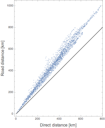
Also interesting is to look at the length of the route versus the direct distance:

copy=DeleteDuplicates[Flatten[#,1]]&/@alldata; (* merge data and delete duplicates*)
directlength=GeoDistance2@@@copy[[All,{1,-1}]]; (* calculate direct distance*)
routelength=BlockMap[GeoDistance2@@#&,#,2,1]&/@copy; (* calculate road distance *)
routelength=Total/@routelength; (* total it*)
ListPlot[{directlength,routelength}\[Transpose]/1000.0,Frame->True,AspectRatio->Automatic,Epilog->{Line[{{0,0},{1000,1000}}]},FrameLabel->(Style[#,14]&/@{"Direct distance [km]","Road distance [km]"})]
Histogram[routelength/directlength,Automatic,"PDF",Frame->True,FrameLabel->(Style[#,14]&/@{"\[CurlyPhi] = Road distance/Direct distance","PDF(\[CurlyPhi])"})]

where GeoDistance2 is a quick version of GeoDistance:

ClearAll[GeoDistance2]
GeoDistance2[{lat1_,lon1_},{lat2_,lon2_}]:=Module[{\[CurlyPhi]1,\[CurlyPhi]2,\[CapitalDelta]\[CurlyPhi],\[CapitalDelta]\[Lambda],a,c},
    {\[CurlyPhi]1,\[CurlyPhi]2}={lat1,lat2}Degree;
    \[CapitalDelta]\[CurlyPhi]=\[CurlyPhi]2-\[CurlyPhi]1;
    \[CapitalDelta]\[Lambda]=(lon2-lon1)Degree;
    a=Haversine[\[CapitalDelta]\[CurlyPhi]]+Cos[\[CurlyPhi]1]Cos[\[CurlyPhi]2]Haversine[\[CapitalDelta]\[Lambda]];
    c=2ArcTan[Sqrt[1-a],Sqrt[a]];
    6.3674446571 10^6c (* result in meters *)
]

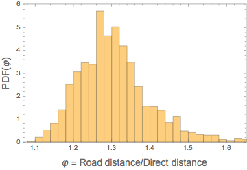
I guess the average ratio describes how developed a country is/how mountainous it is/how many water bodies it has. A comparison for different countries would be very nice. But I don't want to kill the Wolfram servers...

Creating these lines for the routes on a country-scale should be quite easy; just some rotation and scaling. I'll give it a try later. I chose a grid of cities rather than all cities so that it is more homogeneously distributed over the area, and thus not biasing certain areas.

Thanks for the nice comments!

Hi Marco,

Thanks for the kind words. Unfortunately I didn't save the times. But should be also possible. I might try tonight. Just to clarify: I'm also not using the distance now. I just color it by how often a piece of road is 'used' by all the routes. But it might be interesting to see it as a graph indeed. I will dig deeper later...

thanks!