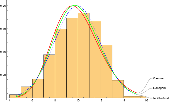
Comparison of Nakagami and Gamma distributions for a list of data

Hi,

I tried to evaluate the Nakagami and Gamma distributions for monthly wind speed data.

Which distribution is better?

How to show two distributions in one plot for comparison.

I appreciate your support and time.

Alex

data = {9.9`, 9.`, 12.7`, 13.3`, 11.3`, 10.`, 9.8`, 8.8`, 8.`, 7.4`, 6.8`, 
   6.8`, 7.1`, 9.4`, 8.4`, 10.`, 15.2`, 11.2`, 9.3`, 9.7`, 8.8`, 8.4`, 6.2`, 
   7.9`, 7.4`, 8.9`, 10.5`, 9.5`, 9.3`, 11.5`, 7.1`, 8.9`, 6.5`, 5.4`, 7.1`, 
   7.6`, 8.8`, 10.2`, 14.7`, 11.9`, 9.9`, 9.8`, 10.8`, 10.2`, 8.6`, 8.9`, 
   8.5`, 8.7`, 8.3`, 10.`, 9.`, 10.5`, 10.2`, 11.5`, 9.6`, 9.9`, 7.8`, 6.8`, 
   7.3`, 5.7`, 7.6`, 5.9`, 7.4`, 8.1`, 9.2`, 10.7`, 9.9`, 9.`, 7.8`, 7.`, 5.`,
    5.7`, 6.4`, 7.1`, 9.7`, 9.9`, 7.3`, 10.7`, 10.7`, 8.2`, 8.2`, 8.8`, 4.7`, 
   5.9`, 7.4`, 6.4`, 8.`, 9.9`, 7.4`, 10.`, 9.3`, 10.8`, 9.6`, 8.6`, 8.4`, 
   8.4`, 7.`, 8.6`, 9.6`, 7.9`, 9.9`, 11.5`, 10.1`, 9.7`, 8.2`, 6.7`, 4.6`, 
   7.5`, 6.`, 7.8`, 9.9`, 10.3`, 8.4`, 10.1`, 11.6`, 12.`, 10.`, 7.9`, 6.5`, 
   5.9`, 10.6`, 9.`, 10.3`, 9.2`, 10.3`, 11.`, 11.2`, 10.4`, 10.3`, 9.5`, 
   8.3`, 10.1`, 8.1`, 9.`, 10.6`, 11.4`, 10.6`, 12.2`, 11.5`, 12.2`, 10.7`, 
   9.4`, 8.2`, 8.5`, 9.3`, 11.3`, 11.5`, 10.3`, 11.`, 12.5`, 12.2`, 12.9`, 
   10.6`, 9.2`, 7.8`, 8.8`, 9.5`, 9.9`, 11.`, 10.9`, 11.7`, 12.8`, 11.4`, 
   13.1`, 12.7`, 10.9`, 9.6`, 10.6`, 10.1`, 12.8`, 11.5`, 11.2`, 11.2`, 11.9`,
    12.2`, 11.3`, 11.2`, 10.`, 8.9`, 7.9`, 8.7`, 11.`, 11.1`, 13.4`, 13.8`, 
   12.5`, 12.1`, 12.`, 10.1`, 10.8`, 8.1`, 10.9`, 9.3`, 11.9`, 12.2`, 11.1`, 
   11.3`, 12.1`, 10.9`, 9.9`, 11.2`, 9.5`, 10.`, 9.9`, 8.6`, 9.6`, 11.3`, 
   11.2`, 11.5`, 11.3`, 10.9`, 10.9`, 10.1`, 10.8`, 8.9`, 6.9`, 9.9`, 10.3`, 
   12.1`, 11.9`, 10.7`, 11.3`, 12.5`, 11.1`, 10.3`, 9.8`, 10.`, 8.8`, 11.3`, 
   10.9`, 12.6`, 11.7`, 11.3`, 11.5`, 12.5`, 11.`, 11.4`, 9.7`, 7.2`, 8.7`, 
   9.8`, 12.6`, 13.2`, 11.8`, 12.2`, 12.4`, 11.5`, 10.2`, 10.3`, 8.1`, 9.7`, 
   7.7`, 8.4`, 10.1`, 13.`, 12.8`, 12.3`, 13.2`, 12.`, 11.6`, 11.8`, 9.`, 
   8.9`, 8.1`, 9.7`, 10.8`, 13.5`, 12.8`, 13.5`, 12.8`, 11.9`, 12.4`, 10.3`, 
   9.5`, 8.4`, 7.7`, 11.4`, 9.8`, 12.8`, 12.4`, 13.1`, 12.5`, 13.1`, 12.3`, 
   9.9`, 8.9`, 8.2`, 6.8`};

(*Gamma Distribution*)

gam = EstimatedDistribution[data, GammaDistribution[\[Alpha], \[Beta]]];

Show[
 Histogram[data, 15, "PDF"],
 Plot[PDF[GammaDistribution[23.81, 0.41], x], {x, Min[data], Max[data]}, 
  Filling -> Axis, Exclusions -> None]]

(*Nakagami Distribution*)

nak = EstimatedDistribution[data, NakagamiDistribution[\[Mu], \[Omega]]];

Show[
 Histogram[data, 15, "PDF"],
 Plot[PDF[NakagamiDistribution[6.39, 102.37], x], {x, Min[data], Max[data]}, 
  Filling -> Axis, Exclusions -> None]]

Hi Alex,

as it seems, Nakagami is slightly better. But if you let the system decide, the NormalDistribution winns:

gam = EstimatedDistribution[data, GammaDistribution[\[Alpha], \[Beta]]];
nak = EstimatedDistribution[data, NakagamiDistribution[\[Mu], \[Omega]]];
best = FindDistribution[data];

plot = Plot[{PDF[gam, x], PDF[nak, x], PDF[best, x]}, {x, Min[data], Max[data]}, PlotStyle -> {Red, Green, {Dashed, Blue}}, PlotLabels -> {"Gamma", "Nakagami", "best:Normal"}];

Show[Histogram[data, Automatic, "PDF"], plot, PlotRange -> {{4, 17.7}, Automatic}, ImageSize -> Large]

Does that help? Regards – Henrik
[1]: https://community.wolfram.com//c/portal/getImageAttachment?filename=distribs.png&userId=32203

Thank you, Henrik.

As you know, we can evaluate these statistics distributions using the AIC.

Where I did I mistake?

(*Maximum Likelihood for Gamma*)

mlegam = 
 FindDistributionParameters[data, GammaDistribution[\[Alpha], \[Beta]]]

(*AIC for Gamma*)

aicgam = -2 LogLikelihood[
    GammaDistribution[{\[Alpha], \[Beta]} /. mlegam], data] + 2*1

(*Maximum Likelihood for Nakagami*)

mlenak = 
 FindDistributionParameters[data, 
  NakagamiDistribution[\[Mu], \[Omega]]]

(*AIC for Nakagami*)

aicnak = -2 LogLikelihood[
    NakagamiDistribution[{\[Mu], \[Omega]} /. mlenak], data] + 2*1

Hi Alex,

There are a couple of syntax errors. Try

aicgam = -2 LogLikelihood[GammaDistribution[\[Alpha], \[Beta]] /. mlegam, data] + 2*1

aicnak = -2 LogLikelihood[NakagamiDistribution[\[Mu], \[Omega]] /. mlenak, data] + 2*1

@RohitNamjoshi and @AlexTeyMouri: Don’t you both want to have 2 * 2 (i.e., 2 * number of estimated parameters) rather than 2 * 1?

Also, is there a real need for a parametric representation of the distribution of the observed data? In other words, why not consider the following?

Show[Histogram[data, "FreedmanDiaconis", "PDF"], SmoothHistogram[data]]

Dear Rohit and Jim,

Thank you so much.

Is it possible to show that SmoothHistogram is better than the Nakagami and Gamma distributions by calculating the AIC values?

With best Regards

Which is best depends on what you mean by “best”, your subject matter, and your objective.

Because you appear to be selecting between a Gamma and a Nakagami distribution, I would assume that there is no theoretical reason for either. As Henrik Schachner demonstrated even a Normal distribution has a smaller AIC value (which is likely involved in FindDistribution.

If the objective is just to summarize the distribution of this particular dataset, then a nonparametric density estimate (i.e., a SmoothHistogram) is what I would recommend. (It’s the 21st century so histograms should not be the first thing to come to mind.)

If there is some appropriate subject matter knowledge or more specific objective is given, then better and more specific advice can be obtained.