Get the inverse Laplace transform of an equation?

[lourdgmassiff (Lucas G)]

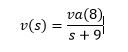
Hi everyone,

I am trying to plot the speed curves of 2 vehicles in Mathematica: the first one (leading vehicle) is a normal vehicle simulating a brutal braking and the second (following vehicle) is an autonomous vehicle that has to react to the first one’s speed variations.
The leading vehicle’s speed curve is easy to get but I ran into a problem regarding the following one. I have the following differential equation in the Laplace domain, with y[s] being the following vehicle’s speed:

I would like to find the equivalent equation in the time domain using Mathematica, but the InverseLaplaceTransform function doesn’t seem to be able to do it (I can’t simply say that s^4*y[s]=y’‘’'[t] because I have boundary conditions in t=0 that are not equal to 0).

If I simplify the equation above in order to express y[s] depending on s, and use the InverseLaplaceTransform function on y[s], it will automatically consider all the boundary conditions equal to zero so I get this result (with the blue curve being the speed (m/s) of the first vehicle depending on time and the yellow curve describing the speed of the following vehicle):

Which is wrong in my case since the following vehicle is already moving (The yellow curve should start at around 15 m/s).

So my questions are: is there a way to specify the boundary conditions to the software when using the InverseLaplaceTransform function? If not, is there a way to convert the equation that I have from the Laplace Domain to the time domain and after that use DSolve to solve the differential equation with the my boundary conditions ?

Sorry if I made any beginner mistakes, I’m quite new to control systems and discovered Mathematica a week ago. Thanks for your advice.

[hdolhaine (Hans Dolhaine)]

Hoe did you get your blue and yellow line.
When I try your way I get

eq =  s^4 y + 19/19 s^3 y + 487/30 s^2 y + 69 s y + 45/10 y == 5 va[8];
yy = y /. Solve[eq, y][[1, 1]]

(* (150 va[8])/(135 + 2070 s + 487 s^2 + 30 s^3 + 30 s^4) *)

and ( with eg. va[8] = 3 )

invLT = InverseLaplaceTransform\[yy, s, t\];
Plot[Evaluate[Re[N[invLT /. va[8] -> 3 /. t -> tt]]], {tt, 0, 25},  PlotRange -> {-30, 30}]]

[hdolhaine (Hans Dolhaine)]

This was the pic I wanted to add

invLT.bmp (80.2 KB)

[lourdgmassiff (Lucas G)]

I don’t have access to Mathematica now so I can’t show you the exact code but the blue curve is the following function in the time domain:

In my example va(8) is around 22.5 m/s.
I obtained the yellow curve by applying InverseLaplaceTransform to this function (which comes from the differential equation):

I notice that your coefficient of s^3 is 30 where it should be 57, maybe the difference comes from this.
[1]: https://community.wolfram.com//c/portal/getImageAttachment?filename=eq1.JPG&userId=1832094
[2]: https://community.wolfram.com//c/portal/getImageAttachment?filename=eq2.JPG&userId=1832094

[neils (Neil Singer)]

Lucas,

You can put initial conditions into the Laplace Transform. To demonstrate this do the following:

teq = y''''[t] + 19/10 y'''[t] + 487/30 y''[t] + 69 y'[t] + 
   45/10 y[t] == 5 va[8]
lap = LaplaceTransform[teq, t, s] // Simplify    

Note that the derivatives you want to set are explicitly in the equation. Set the initial conditions:

tosolve = 
Solve[lap, LaplaceTransform[y[t], t, s]][[1]] /. { va[8] -> 225/10, 
y[0] -> 10, y'[0] -> 1, y''[0] -> 0, y'''[0] -> 0}

(*   {LaplaceTransform[y[t], t, s] -> (
3375 + 21187 s + 4927 s^2 + 600 s^3 + 300 s^4)/(
s (135 + 2070 s + 487 s^2 + 57 s^3 + 30 s^4))} *)

In[4]:= invLT = InverseLaplaceTransform[tosolve, s, t] // Simplify;

In[5]:= Chop[invLT /. t -> 0 // N]

Out[5]= {y[0] -> 10.}

When I plot the result it has the correct initial conditions however its unstable but I don’t know the origin of your equations so I can’t speak to that.
I hope this helps.

Regards,

Neil

[anon21378091]

That’s what I was looking for. Thank you, I will try it when I can.

[hdolhaine (Hans Dolhaine)]

You are right, there is a typo in my post.

But

eq =  s^4 y + 19/10 s^3 y + 487/30 s^2 y + 69 s y + 45/10 y == 5 va[8];
yy = y /. Solve[eq, y][[1, 1]]

 ( *  (150 va[8])/(135 + 2070 s + 487 s^2 + 57 s^3 + 30 s^4)  *)

this gives the same peculiar Plot ( perhaps Neil means this as unstable behaviour) as before, even with 57 as coefficient of s^3.

There is another remark. You are looking for a differential equation in the t-domain which gives your equation in the s-domain. Independent of the initial values of f what do you say to this (but I don’t have any idea how to handle such an equation)

dgl = 9/2 y DiracDelta[t] + 69 DiracDelta[t] f[0] - 
  5 DiracDelta[t] va[8] + 487/30 f[0] 
\!\(\*SuperscriptBox["DiracDelta", "\[Prime]",
MultilineFunction->None]\)[t] + 487/30 DiracDelta[t] 
\!\(\*SuperscriptBox["f", "\[Prime]",
MultilineFunction->None]\)[0] + 19/10 
\!\(\*SuperscriptBox["DiracDelta", "\[Prime]",
MultilineFunction->None]\)[t] 
\!\(\*SuperscriptBox["f", "\[Prime]",
MultilineFunction->None]\)[0] + 69 
\!\(\*SuperscriptBox["f", "\[Prime]",
MultilineFunction->None]\)[t] + 19/10 f[0] 
\!\(\*SuperscriptBox["DiracDelta", "\[Prime]\[Prime]",
MultilineFunction->None]\)[t] + 
\!\(\*SuperscriptBox["f", "\[Prime]",
MultilineFunction->None]\)[0] 
\!\(\*SuperscriptBox["DiracDelta", "\[Prime]\[Prime]",
MultilineFunction->None]\)[t] + 19/10 DiracDelta[t] 
\!\(\*SuperscriptBox["f", "\[Prime]\[Prime]",
MultilineFunction->None]\)[0] + 
\!\(\*SuperscriptBox["DiracDelta", "\[Prime]",
MultilineFunction->None]\)[t] 
\!\(\*SuperscriptBox["f", "\[Prime]\[Prime]",
MultilineFunction->None]\)[0] + (487 
\!\(\*SuperscriptBox["f", "\[Prime]\[Prime]",
MultilineFunction->None]\)[t])/30 + f[0] 
\!\(\*SuperscriptBox["DiracDelta", 
TagBox[
RowBox[{"(", "3", ")"}],
Derivative],
MultilineFunction->None]\)[t] + DiracDelta[t] 
\!\(\*SuperscriptBox["f", 
TagBox[
RowBox[{"(", "3", ")"}],
Derivative],
MultilineFunction->None]\)[0] + 19/10 
\!\(\*SuperscriptBox["f", 
TagBox[
RowBox[{"(", "3", ")"}],
Derivative],
MultilineFunction->None]\)[t] + 
\!\(\*SuperscriptBox["f", 
TagBox[
RowBox[{"(", "4", ")"}],
Derivative],
MultilineFunction->None]\)[t]

(That looks somewhat weird, just copy and paste it, it can for sure be better written))

Then the LaplaceTransform is essentially your equation ( with the 5 va[8] term on the left side)

In[17]:= eq4 =  Expand[LaplaceTransform[dgl, t, s] /.  LaplaceTransform[f[t], t, s] -> y]

Out[17]= (9 y)/2 + 69 s y + (487 s^2 y)/30 + (19 s^3 y)/10 + s^4 y -  5 va[8]

[hdolhaine (Hans Dolhaine)]

I just noticed that simple copy and paste with the expression above didn’t work, at least on my system. So here another version.

Your equation in the s - domain

eq = s^4 y[s] + 19/10 s^3 y[s] + 487/30 s^2 y[s] + 69 s y[s] + 45/10 y[s] - 5 va[8];

Let

dgl1 = f''''[t] + 19/10 f'''[t] + 487/ 30 f''[t] + 69 f'[t] +   45/10 f[t] - 5 va[8] DiracDelta[t];

be a 1st attempt in the t-domain. But this doesn’t yield your equation after the LaplaceTransform.
So calculate

xx = (LaplaceTransform[dgl1, t, s] - eq) /. LaplaceTransform[f[t], x__] -> y[s];
yy = InverseLaplaceTransform[xx, s, t];
zz = dgl1 - yy;
eq1 = LaplaceTransform[zz, t, s] /. LaplaceTransform[f[t], x__] -> y[s];
eq1 - eq // Simplify

then zz is the differential equation in the t-domain yielding the complicated output from above in a more convenient form and giving your equation in the s - domain.

[lourdgmassiff (Lucas G)]

It’s a good way to solve it, I will also try it, thank you !