I'm having problems with third type heat transfer boundary condition

Hi! I’m a beginner level user of Mathematica, and still learning it. Basically, I’m trying to monitor the natural cooling of an imaginary plastic slab with the top/bottom side insulated, only the left/right side is dissipating heat to the environment. Thus the model reduced to a 1D heat transfer model. The slab has a thickness of 10mm, and initial uniform temperature of 275C, the environment temperature is 25C. I’m trying to implement a Neumann type boundary condition at both left (x = -5) and right (x = 5) side, i.e., k*dT/dx = h(T-Tenvironment) at boundary, but I keep getting error messages that the boundary and initial conditions are inconsistent and more importantly the results looks unstable, my code looks like this, can anyone give me a little help? Would be really appreciated!

h = 13/(1000^2);(*units are converted to mm*)
k = 0.3/1000;
c = 1030;
rou = 1380/(1000^3);
heq = rou*c*D[u[t, x], t] == k*D[u[t, x], {x, 2}];
ic = u[0, x] == 275;
bcs1 = (D[u[t, x], x] /. x -> 5) + h*(u[t, 5] - 25) == 0;
bcs2 = (D[u[t, x], x] /. x -> -5) + h*(u[t, -5] - 25) == 0;
sol = NDSolve[{heq, ic, bcs1, bcs2}, u[t, x], {t, 0, 20}, {x, -5, 5}];
F[t_, x_] = u[t, x] /. sol[[1]];
Plot3D[F[t, x], {x, -5, 5}, {t, 0, 15}, PlotRange -> All, 
 AxesLabel -> Automatic]

Untitled-3.nb (212 KB)
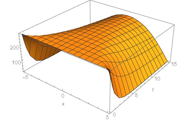
NDSolve is full of mysteries. I learnt that sometimes forcing something to be zero for a (very) short time can help.
You could try this.

h = 13/(1000^2);(*units are converted to mm*)k = 0.3/1000;
c = 1030;
rou = 1380/(1000^3);
heq = rou*c*D[u[t, x], t] == k*D[u[t, x], {x, 2}];
ic = u[0, x] == 275;
bcs1 = (D[u[t, x], x] /. x -> 5) == -h*(u[t, 5] - 25) (1 - Exp[-30 t]);
bcs2 = (D[u[t, x], x] /. x -> -5) == 
   h*(u[t, -5] - 25) (1 - Exp[-30 t]);
sol = NDSolve[{heq, ic, bcs1, bcs2}, u[t, x], {t, 0, 20}, {x, -5, 5},
   Method -> {"MethodOfLines", 
     "SpatialDiscretization" -> {"TensorProductGrid", 
       "MinPoints" -> 100}}];
F[t_, x_] = u[t, x] /. sol[[1]];
Plot3D[F[t, x], {x, -5, 5}, {t, 0, 15}, PlotRange -> All, 
 AxesLabel -> Automatic]

Hi Hans! Thank you so much for your help! But unfortunately, it still didn’t work. So strangely, by implementing boundary conditions like this:

bcs1 = D[u[t, 5], x] == -h*(u[t, 5] - 25), 
bcs2 = D[u[t, -5], x] == -h*(u[t, -5] - 25)

the result looks reasonable. It looks like this:

with the temperature at left/right side gradually decreasing. BUT I also learned from somewhere else that it’s incorrect to implement boundary conditions like this:

D[u[t, 5], x] == -h*(u[t, 5] - 25)

because in D[u[t, 5], x], the u[t, 5] is no longer a function of x, so instead the derivative in boundary condition should be like D[u[t, x], x] /. x → 5.
With the boundary condition like D[u[t, x], x] /. x → 5, I tried what you suggested, but unfortunately, the result still looks erroneous

may I ask if you can give me some more help on this? I’m really appreciated for your help!

I don’t know what is happening. I attach a notebook with my code, look at the plot (before running the notebook). It contains D[u[t, x], x] /. x → 5, and gives a reasonalbe result.

diffbarnum2sides.nb (73.9 KB)

Hi Hans! I’m not sure what happened wither, probably different versions of Mathematica? I ran your code and the same wierd result replaced your original one, but when I increase the MinPoints from 100 to 200 it worked! Thank you!

Super. As I said: NDSolve is full of mysteries. I have Version 7. And I think there is a theoretical solution to your problem, albeit in form of an infinite series. You may want to have a look in these books

Frieder Häfner, Dietrich Sames, Hans-Dieter Voigt, Wärme- und Stofftransport
Springer Verlag, Berlin 1992

https://www.amazon.de/s?k=frieder+häfner+wärme&__mk_de_DE=ÅMÅŽÕÑ&ref=nb_sb_noss

Horatio Scott Carslaw, John Conrad Jaeger, Conduction of Heat in Solids, 2nd Edition
Oxford Science Publications, Oxford University Press 1959

Both contain lots of solved problems.

In the 2nd part of the attached notebook ( after the 1st line of stars ) you will find an example (although with different values compared to your problem) how to find that series which is a solution to your problem using the method of Laplace-Transforms. I did it only for 0 <= x <= 5, as the problems is symmetric with respect to x.

If you have any question concerning the method please feel free to contact me.

Regards Hans

diffbarnum2sides.nb (305 KB)

I did some more work on this problem. See the attached notebook.

diffbarnum2sides-a.nb (755 KB)

Hans, I’m so grateful for your help!! Learned a lot from reading the notebooks you send me!