NDSolve error: step size is effectively zero

I am trying to solve a nonlinear differential equation using NDSolve

numericaldiffeqqa = 
NDSolve[{(q^\[Prime]\[Prime])[\[Phi]] + q[\[Phi]] == -(
1/(1 + q[\[Phi]])^2), q[0] == 1, q'[0] == 1}, 
q, {\[Phi], 0, 50}];

Plot[Evaluate[q[\[Phi]] /. numericaldiffeqqa], {\[Phi], 0, 50}, 
PlotRange -> All]

ParametricPlot[
Evaluate[{q[\[Phi]], q'[\[Phi]]} /. numericaldiffeqqa], {\[Phi], 0, 
50}]

gives the result of

NDSolve::ndsz: At \[Phi] == 2.5326866484431907`, step size is effectively zero; singularity or stiff system suspected.

What do I do to fix this?

Lance,

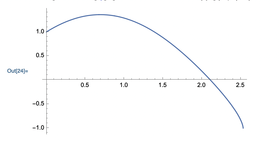
The error is real. Your equations have a singularity just over Phi = 2.532687. Do the following:

numericaldiffeqqa = 
  NDSolve[{q''[\[Phi]] + q[\[Phi]] == -(1/(1 + q[\[Phi]])^2), 
    q[0] == 1, q'[0] == 1}, q, {\[Phi], 0, 2.532687}, 
   Method -> "StiffnessSwitching"];

Plot[Evaluate[q[\[Phi]] /. numericaldiffeqqa], {\[Phi], 0, 2.532687}, 
 PlotRange -> All]

and you get this:

Note that q[phi] goes to -1. Your differential equation has a divide by zero if q[phi] is -1.

Regards

Neil
[1]: https://community.wolfram.com//c/portal/getImageAttachment?filename=ScreenShot2021-11-27at12.05.15AM.png&userId=599067

Lance,

You can’t integrate through the singularity – the solution makes no sense because the derivative, q’'[phi] goes to -Infinity at that point. You need to understand what you are trying to solve and determine why the equations blow up. Maybe you set poor initial conditions, maybe you have the wrong equations.

Regards

We can expand range from singular point at phi=2.532687 to another singular point at phi=6.207986.

singularpoint = Rationalize[2.532687, 0];
numericaldiffeqqa = 
  NDSolve[{q''[\[Phi]] + q[\[Phi]] == -(1/(1 + q[\[Phi]])^2), 
    q[0] == 1, q'[0] == 1, 
    WhenEvent[\[Phi] == singularpoint, 
     q'[\[Phi]] -> Abs[q'[\[Phi]]]]}, q, {\[Phi], 0, 7}, 
   WorkingPrecision -> 20];
Plot[Evaluate[q[\[Phi]] /. numericaldiffeqqa], {\[Phi], 0, 7}]

eq = q''[\[Phi]] + q[\[Phi]] + (1/(1 + q[\[Phi]])^2);(*eq = 0*)
Plot[Evaluate[eq /. numericaldiffeqqa], {\[Phi], 0, 7}](*Almost zero. Solution are correct*)

Mariusz,

I like your approach of symmetrically jumping over the singularity (fix the q’[x] to the absolute value and restart from there). Its clever.

I’m curious, What would be the physical meaning of that solution? Is it connected to the first solution in any way? Or is it just a reflection across the singularity?

Regards.

Thank you Neil, this was very helpful. Is there a way to plot the values after 2.532687 in order to continue the plot?

Regards Lance

Marius, this is a good way of resolving the singularities in the numerical solution. The parametric plot of the solution almost makes an orbit. Is there a way to extend the solution even further for every singularity?