Numerical solution of fourth order differential equation

Could you tell me to solve numerically the equation with the next boundary conditions

\[Pi]^4 Y[y] - b^4 N0 (Y^\[Prime]\[Prime])[y] - 
  2 b^2 \[Pi]^2 (Y^\[Prime]\[Prime])[y] + 
  b^3 N0 y \[Alpha] (Y^\[Prime]\[Prime])[y] + b^4 
\!\(\*SuperscriptBox[\(Y\), 
TagBox[
RowBox[{"(", "4", ")"}],
Derivative],
MultilineFunction->None]\)[y] == 0
Y[0] == 0;
Y[1] == 0;
Y''[0] == 0;
Y''[1] == 0;

Hi,

there are quite some issues with that. First of all there are many free parameters such b, N0, \alpha. To integrate numerically you need to substitute values for them (or use ParametricNDSolve). Syntax that produces an output is:

sols = NDSolve[{\[Pi]^4 Y[y] - b^4 N0 (Y^\[Prime]\[Prime])[y] - 
      2 b^2 \[Pi]^2 (Y^\[Prime]\[Prime])[y] + 
      b^3 N0 y \[Alpha] (Y^\[Prime]\[Prime])[y] + 
      b^4 D[Y[y], {y, 4}] == 0 /. {b -> 1., N0 -> 1, \[Alpha] -> 1},
   Y[0] == 0, Y[1] == 0, Y''[0] == 0, Y''[1] == 0}, Y[y], {y, 0, 1}]

There might be some numerical issues though because

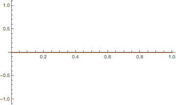
Plot[Y[y] /. sols, {y, 0, 1}]

gives

which is numerically zero, where it should be plainly zero. You can fix this by setting a higher Accuracy Goal:

sols = NDSolve[{\[Pi]^4 Y[y] - b^4 N0 (Y^\[Prime]\[Prime])[y] - 
      2 b^2 \[Pi]^2 (Y^\[Prime]\[Prime])[y] + 
      b^3 N0 y \[Alpha] (Y^\[Prime]\[Prime])[y] + 
      b^4 D[Y[y], {y, 4}] == 0 /. {b -> 1., N0 -> 1, \[Alpha] -> 1},
   Y[0] == 0, Y[1] == 0, Y''[0] == 0, Y''[1] == 0}, Y[y], {y, 0, 1}, 
  AccuracyGoal -> 100]

That gives a flatline zero.

Cheers,

Marco

Here is what you can try. I believe this time Mathematica hasn’t found a non-trivial solution yet. You may try give this equation a reasonable choice of parameters:

But all the deviations from zero that you see, are only numerical artefacts, aren’t they?

sols = ParametricNDSolve[{\[Pi]^4 Y[y] - 
     b^4 N0 (Y^\[Prime]\[Prime])[y] - 
     2 b^2 \[Pi]^2 (Y^\[Prime]\[Prime])[y] + 
     b^3 N0 y \[Alpha] (Y^\[Prime]\[Prime])[y] + 
     b^4 D[Y[y], {y, 4}] == 0,
   Y[0] == 0, Y[1] == 0, Y''[0] == 0, Y''[1] == 0}, 
  Y, {y, 0, 1}, {N0, b, \[Alpha]}, AccuracyGoal -> 100]

gives

I suppose that the existence and uniqueness theorem would suggest that there is only one solution, which is the “trivial” solution?

Cheers,

M.

PS: Another clue that the solutions that deviate from zero cannot be accurate is that they do not fulfil one of the boundary conditions, i.e. Y1==0.

You are right. These deviations are just either numerical error or internal values.

If you modify the boundary conditions, the solver gives the reasonable solution. I guess in your case the solution is very likely Y[x] == 0.

Thank you very much.
I did not know about “AccuracyGoal”.
I’m solving an equation of elastic buckling of rectangular plate with linearly varying in-plane load and I expected the solution similar to Y[y] = Sin[[Pi]*y/b]. This is the solution of my equation if [Alpha] = 0 and load is constant. I expected solution similar to the last picture.