DOWNLOAD-DESKTOP-NOTEBOOK.nb (2.07 MB)
 – you have earned Featured Contributor Badge

Your exceptional post has been selected for our editorial columns Staff Picks http://wolfr.am/StaffPicks and Publication Materials https://wolfr.am/PubMat and Your Profile is now distinguished by a Featured Contributor Badge and is displayed on the Featured Contributor Board. Thank you!
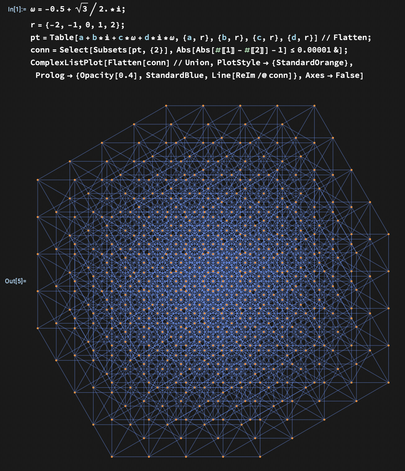
The following code reconstructs the graphics above:
\[Omega]=-0.5+Sqrt[3]/2.*I;
r={-2,-1,0,1,2};
pt=Table[a+b*I+c*\[Omega]+d*I*\[Omega],{a,r},{b,r},{c,r},{d,r}]//Flatten;
conn=Select[Subsets[pt,{2}],Abs[Abs[#[[1]]-#[[2]]]-1]<=0.00001&];
ComplexListPlot[Flatten[conn]//Union,PlotStyle->{StandardOrange},
Prolog->{Opacity[0.4],StandardBlue,Line[ReIm/@conn]},Axes->False]
Great – thanks for sharing!
The code here reconstructs the exact same optimal configuration shown on the right-hand side of this Twitter/X post using Moser ring:
\[Alpha]=N@Exp[I*ArcCos[1/2]];
\[Beta]=N@Exp[I*ArcCos[5/6]];r=Range[-2,2];
pt2=Select[Table[a+b*\[Alpha]+c*\[Beta]+d*\[Alpha]*\[Beta],{a,r},{b,r},{c,r},{d,r}]//Flatten,Abs[#]<=4.&];
f=Nearest[pt2,Method->Automatic];
lines=Flatten[
Table[With[{pool=f[ele,{All,4}]},{ele,#}&/@Select[pool,Abs[EuclideanDistance[#,ele]-1.]<0.0001&]],{ele,pt2}],1];
conn=Union[Sort/@lines];
vtx=Flatten[conn]//Union;
ComplexListPlot[vtx,PlotStyle->{StandardOrange},PlotStyle->Tiny,Prolog->{Opacity[0.4],StandardBlue,Line[ReIm/@conn]},Axes->False,PlotRangePadding->0]
This is great! Note, this plot was featured in Nature news:
AI cracks 80-year-old mathematics challenge — researchers are astonished
DOI: AI cracks 80-year-old mathematics challenge — researchers are astonished | Nature
Looks like this is quite minimal implementation of that plot in Wolfram:
p=Tuples[Range[-2,2],4] . I^{0,1,4/3,7/3};
RelationGraph[Abs[#1-#2]==1&,p,VertexCoordinates->ReIm@p]
adding VertexStyle->Red renders this:
Here is a paper that presents an experimental approach of the problem and disproves the initial conjecture.