Introduction
In a previous post, Copulas in Risk Management, I covered the theory and applications of copulas in the area of risk management, pointing out the potential benefits of the approach and how it could be used to improve estimates of Value-at-Risk by incorporating important empirical features of asset processes, such as asymmetric correlation and heavy tails.
In this post I take a different tack, to show how copula models can be applied in pairs trading and statistical arbitrage strategies.
This is not a new concept - it stems from when copulas began to be widely adopted in financial engineering, risk management and credit derivatives modeling. But it remains relatively under-explored compared to more traditional techniques in this field. Fresh research suggests that it may be a useful adjunct to the more common methods applied in pairs trading, and may even be a more robust methodology altogether, as we shall see.
Traditional Approaches to Pairs Trading
Researchers often use simple linear correlation or distance metrics as the basis for their statistical arbitrage strategies. The problem is that statistical relationships may be nonlinear or nonstationary. Correlations (and betas) that have fluctuated in a defined range over a considerable period of time may suddenly break down, producing substantial losses.
A more sophisticated technique is the Kalman Filter, which can be used as a means of dynamically updating the the estimated correlation or relative beta between pairs (or portfolios) of stocks, a technique I have written about in the post Statistical Arbitrage with the Kalman Filter.
Another commonly employed econometric technique relies on cointegration relationships between pairs or small portfolios of stocks, as described in my post on Developing Statistical Arbitrage Strategies Using Cointegration. The central idea is that, in theory, cointegration is a more stable and reliable basis for assessing the relationship between stocks than correlation.
Researchers often use a combination of methods, for example by requiring stocks to be both cointegrated and with stable, high correlation throughout the in-sample formation period in which betas are estimated.
In all these cases, however, the challenge is that, no matter how they are derived or estimated, statistical relationships have a tendency towards instability. Even a combination of several of these methods often fails to detect signs of a breakdown in statistical relationships. There is even evidence that cointegration models are no more robust or reliable than simple correlations. For example, in his paper On the Persistence of Cointegration in Pairs Trading, Matthew Clegg assess the persistence of cointegration among U.S. equities in the calendar years 2002-2012, comprising over 860,000 pairs in total. He concludes that the evidence does not support the hypothesis that cointegration is a persistent property.
Pairs Trading in the S&P500 and Nasdaq Indices
To illustrate the copula methodology I will use an equity pair comprising the S&P 500 and Nasdaq indices. These are not tradable assets, but the approach is the same regardless and will serve for the purposes of demonstrating the technique.
We begin by gathering daily data on the indices and calculating the log returns series. We will use the data from 2010 to 2015 as the in-sample formation period, and test the strategy out of sample on data from Jan 2016-Feb 2017.

The chart below shows a scatter plot of daily percentage log returns on the SP500 and NASDAQ indices.

MODELING
Marginal Distribution Fitting
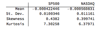
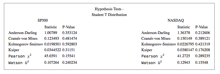
In the post Copulas in Risk Management it was shown that the returns series for the two indices were well-represented by Student T distributions. I replicate that analysis here, estimating the parameters by maximum likelihood and proceed from there to test each distribution for goodness of fit. In each case, the Student T distribution appears to provide an adequate fit for both series.


Copula Calibration
We next calibrate the parameters for the Gaussian copula by maximum likelihood, from which we derive the joint distribution for returns in the two indices via Sklars decomposition. This will be used directly in the pairs trading algorithm. As pointed out previously, there are several alternatives to MLE, including the Method of Moments, for example, and these are listed in the Mathematica documentation for the EstimatedDistrubution function. 


Pairs Trading with the Copula Model
Once we have successfully fitted marginal distributions for the two series and a copula distribution to describe their relationship, we are able to derive the joint distribution. This means that we can directly calculate the joint probability of each pair of data observations. So, for instance, we find that the probability of a return in the S&P500 of 5% or more, together with a return in the Nasdaq of 1% or higher, is approximately 0.2%:


So the way we test our model is to calculate the daily returns for the two indices during the-out-of sample period from Jan 2016 to Feb 2017 and compute the probability of each pair of daily observations. On days where we see observation pairs with abnormally low estimated probabilities, we trade the pair accordingly over the following day.
Naturally, there are multiple issues with this simplistic approach. To begin with, the indices are not tradable and if they were we would have to account for transaction costs including the bid-offer spread. Then there is the issue of determining where to set the probability threshold for initiating a trade. We also need to decide on criteria to try to optimize the trade holding period or trade exit rules. And, finally, we need to think about trade expression: for example, we might attempt to trade both legs passively, perhaps crossing the spread to fill the remaining leg when an order for one of the pairs is filled.
But none of these issues are specific to the copula approach - they apply equally to all of the methods discussed previously. So, for the sake of clarity, I am going to ignore them. In this analysis I pick a threshold probability level of 15% and assume we hold the trade for one day only, opening and closing the trade at the start and end of the day after we receive a signal. In computing the returns for each trade I ignore any transaction costs.
First, we gather data for the test period:
Next, we use the estimated joint distribution to compute the probability of each daily observation of index returns. We gather the daily returns series and associated probability series into a single temporal variable:


We plot the time series of index returns and associated probabilities as follows:


Trade Signal Generation
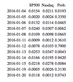
The table below lists the index returns and joint probabilities over the first several days of the series. The sequence of trade signals is as follows:
After a very low probability reading for 2016/1/4, we take equally weighted positions short the S&P500 Index and long the Nasdaq index on 2016/1/5. We close the position at the end of the day, producing a total return of 0.44%. Similar signals are generated on 2016/1/6, 2016/1/7, 2016/1/8, 2016/1/13 , 2016/1/15 and 2016/1/20 (assuming a 15% probability threshold). We take the reverse trade (Buy the S&P500, Sell the Nasdaq) on only one occasion in the initial part of the sample, on 2016/1/14.

Pairs Trading Strategy Results
We are now ready to apply the trading algorithm to the entire sample and chart the resulting P&L.


Comment on Strategy Performance
The performance of the strategy over the out-of-sample period, at just under 4%, can hardly be described as stellar. But this is largely due to the dampening of volatility seen in both indices over the last year, which is reflected in the progressively lower volatility of joint probabilities over the course of the test period. Such variations in signal frequency and trading strategy performance are commonplace in any statistical arbitrage strategy, regardless of the methodology used to generate the signals.
The obvious remedy is to create similar trading algorithms for a large number of pairs and combine them together in an overall portfolio that will produce a sufficient number of signals and trading opportunities to make the performance sufficiently attractive. One of the benefits of statistical arbitrage strategies developed in this way is their highly efficient use of capital, since the combination of long and short positions minimizes the margin requirement for each trade and for the portfolio as a whole.
Finally, it is worth noting here that, in principle, one could easily create similar copula-based arbitrage strategies for triplets, quadruplets, or any (reasonably small) number of assets. The principle restriction lies in the increasing difficulty of estimating the copulas and joint densities, given the slow convergence of the MLE method.
Recent Research
In the last few years several researchers have begun exploring the application of copulas as a basis for statistical arbitrage. In their paper Nonlinear dependence modeling with bivariate copulas: Statistical arbitrage pairs trading on the S&P 100, Krauss and Stubinger apply the copula approach to pairs drawn from the universe of S&P 100 index constituents, with promising results. They conclude that their findings pose a severe challenge to the semi-strong form of market efficiency and demonstrate a sophisticated yet profitable alternative to classical pairs trading.
In the paper by Rad, et al., cited below, the researchers compare several different methods for pairs trading strategies. They find that all of the tested methods produce economically significant returns, but only the performance of the copula-based approach remains consistent after 2009. Further, the copula method shows better performance for its unconverged trades compared to those of the other methods.
Conclusion
The application of copulas to statistical arbitrage strategies is an interesting and relatively under-explored alternative to the usual distance and correlation based methods. In addition to its sound theoretical underpinnings, the copula approach appears to offer greater consistency in performance compared to traditional techniques, whose efficacy has declined since the financial crisis on 2008/09. The benefits of the approach must be weighed against its greater computational complexity, although with the growth in the power of modeling software in recent years this represents less of an obstacle than it has previously.
References
Clegg., M., , On the Persistence of Cointegration in Pairs Trading, Jan. 2014
Krauss, C. and Stubinger , J., Nonlinear dependence modeling with bivariate copulas: Statistical arbitrage pairs trading on the S&P 100, Institut für Wirtschaftspolitik und Quantitative Wirtschaftsforschung, No 15/2015.
Rad, H., Kwong, R., Low, Y. and Faff, R., The profitability of pairs trading strategies: distance, cointegration, and copula methods, Quantitative Finance, DOI: org/10.1080/14697688.2016.1164337, 2015


