This is a call for some feedback on a small utility function I am trying to design. A few times I felt the need in a continuous partitioning of space. Could you please, after reading the post, give me some feedback on:

• What other applications this function can be used for? (Especially higher-dimensional cases)
• Do you have a better design suggestions?

Definition

The SpacePartition function is a continuous analog of Partition. It subdivides n-dimensional space into integer number of partitions. The result is a tensor of hyper-blocks spanning the hyperspace without gaps or overlaps. It means currently, and for simplicity of the demo, there are no block offsets, but they could be added in the future.

SpacePartition[space_List, partitions_List] :=
  Outer[List, ##, 1] & @@ MapThread[Partition[Subdivide @@ Append[#1, #2], 2, 1] &, {space, partitions}]

1D Examples

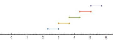
Subdividing 1D interval {2.3,5.7} into 5 consecutive intervals:

part1D = SpacePartition[{{2.3, 5.7}}, {5}]

{{{2.3, 2.98}}, {{2.98, 3.66}}, {{3.66, 4.34}}, {{4.34, 5.02}}, {{5.02, 5.7}}}

NumberLinePlot[Interval @@@ part1D]

2D Examples

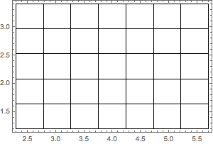
Subdividing 2D rectangle into different number of partitions along different dimensions

part2D = SpacePartition[{{2.3, 5.7}, {1.2, 3.4}}, {7, 5}];

and visualizing as a grid

Graphics[grid2D = {FaceForm[], EdgeForm[Black], Rectangle @@ Transpose[#]} & /@ 
Flatten[part2D, 1], Frame -> True]

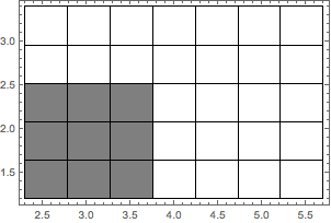
Subdivisions preserve the neighborhood structure

Graphics[{grid2D, {Opacity[.5], Rectangle @@ Transpose[#]} & /@ 
(part2D[[##]] & @@@ Tuples[{1, 2, 3}, 2])}, Frame -> True]

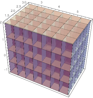
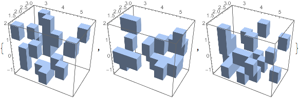
3D Examples

Subdividing 3D rectangle into different number of partitions along different dimensions

part3D = SpacePartition[{{2.3, 5.7}, {1.2, 3.4}, {-1.1, 2}}, {7, 5, 4}];

and visualizing as a 3D grid

Graphics3D[{Opacity[.6], Cuboid @@ Transpose[#]} & /@ Flatten[part3D, 2], Axes -> True]

Selecting random subsets of subdivisions as Region:

Table[Show[Region[Cuboid @@ Transpose[#]] & /@ 
RandomSample[Flatten[part3D, 2], 20], Axes -> True, Boxed -> True],3]

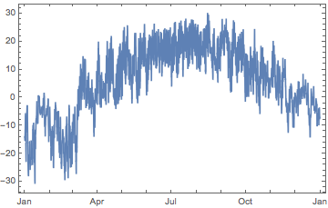
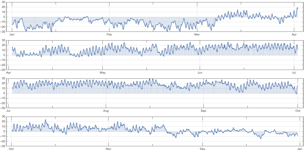
Application: quarterly temperatures or partitioning PlotRange

Often data are so dense it is hard to distinguish details in a standard plot.

data = WeatherData["KMDZ", "Temperature", {{2015}}];
plot = DateListPlot[data]

SpacePartition can be used to partition PlotRange and make a better visual

With[{pr = PlotRange /. Options[plot]},
  DateListPlot[TimeSeriesWindow[data, #], AspectRatio -> 1/10, ImageSize -> 1000,
     PlotRange -> {Automatic, {-30, 30}}, Filling -> Axis, PlotTheme -> "Detailed"] & /@
      Map[DateList, Flatten[SpacePartition[{pr[[1]]}, {4}], 1], {2}]] // Column

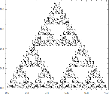
Application: box-counting method for fractal measures

Define an iterated function system (IFS) and iterate it on point sets

IFS[{T__TransformationFunction}][pl_List] := Join @@ Through[{T}[pl]]
IFSNest[f_IFS, pts_, n_Integer] := Nest[f, pts, n]

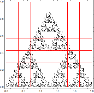
Sierpi?ski gasket transformation:

SierpinskiGasket = With[{\[ScriptCapitalD] = DiagonalMatrix[{1, 1}/2]},
   IFS[{AffineTransform[{\[ScriptCapitalD]}], 
     AffineTransform[{\[ScriptCapitalD], {1/2, 0}}], 
     AffineTransform[{\[ScriptCapitalD], {0.25, 0.433}}]}]];

and corresponding iterated point set

ptsSierp = IFSNest[N@SierpinskiGasket, RandomReal[1, {100, 2}], 4];
graSierp = Graphics[{PointSize[Tiny], Point[ptsSierp]}, Frame -> True]

Function that makes partitions

blocks[n_]:=Rectangle@@Transpose[#]&/@Flatten[N@SpacePartition[{{0,1},{0,1}},{n,n}],1]

Show[graSierp,Graphics[{FaceForm[],EdgeForm[Red],blocks[7]}]]

Of course number of partitions grows as a square for 2D case

Length /@ blocks /@ Range[9]

{1, 4, 9, 16, 25, 36, 49, 64, 81}

Function counting partitions that have any points in them

blockCount[pts_, n_] := Length[Select[blocks[n], MemberQ[RegionMember[#, pts], True] &]]

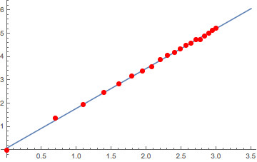
Accumulating data of partition count for different partition sizes

logMes = ParallelTable[Log@{k, blockCount[ptsSierp, k]}, {k, 20}];

Fitting the log-log scale of the data linearly with the slope measuring fractal dimension

fit[x] = Fit[logMes, {1, x}, x]

0.0884774 + 1.70962 x

which deviates a bit from ideal due to probably random inexact nature of IFS system

N[Log[3]/Log[2]]

1.58496

Plot[fit[x], {x, 0, 3.5}, Epilog -> {Red, PointSize[.02], Point[logMes]}]

Missing features

The following features could be added in future:

• Offset parameter for overlapping or gapped partitions

• Real (non-integer) number of partitions