This community post accompanies my Wolfram blog post How Optimistic Do You Want to Be? Bayesian Neural Network Regression with Prediction Errors , so if you find the following interesting, please give that a read as well.

In the documentation there is a tutorial about doing neural network regression with uncertainty. This approach works under certain circumstances, but it can be difficult to generalize, so I started looking for other ways to do it.

As it turns out, there is a link between regression neural networks and Gaussian processes which can be exploited to put error bands on the predictions (see, e.g., this post by Yarin Gal; his thesis and the PhD thesis by R.M. Neal 1995). The basic idea here is to use the DropoutLayer to create a noisy neural network which can be sampled multiple times to get a sense of the errors in the predictions (though it's not quite as simple as I'm making it sound here).

Inspired by Yarin's post above and his interactive example of a network that is continuously being retrained on the example data, I decided to do something similar in Mathematica. The result is the code below, which generates an interactive example in which you can edit the network's training data (by clicking in the figure) and adjust the network parameters with controls. I had some trouble getting the code to not cause strange front end issues, but it seems to work quite well now.

In the attached notebook I go into a bit more detail of my implementation of this method and also show how to do regression with a non-constant noise level. I hope this is of some use to anyone here :)

Example 1: fitting with a network that assumes a constant noise level (mean + 1 sigma error bars)

Example 2: fitting with a network that fits the noise level to the data (heteroscedastic regression)

Homoscedastic regression

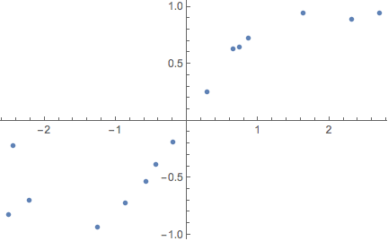
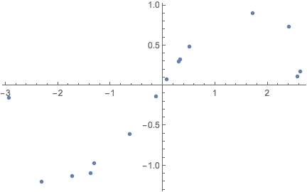
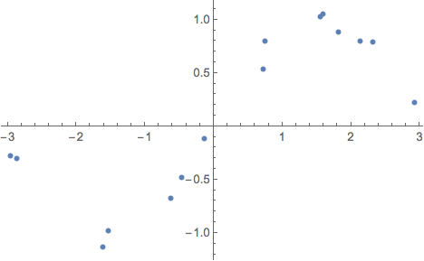
First generate some training examples:

exampleData = Table[{x, Sin[x]} + RandomVariate[NormalDistribution[0, .15]], 
   {x, RandomVariate[UniformDistribution[{-3, 3}], 15]}];
ListPlot[exampleData]

In homoscedastic regression, the noise level of the data is assumed constant across the x-axis. To calibrate the model, you need to provide a prior length scale l that expresses your belief in how correlated the data are over distance (just like in Gaussian process regression). Together with the L2 regularisation coefficient Subscript[λ, 2]; the dropout probability p and the number of training data points N, you have to add the following variance to the sample variance of the network:

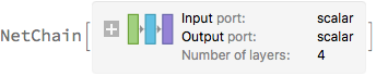
For demonstration purposes, we'll be using a net with one non-linearity. If you want to use more, you need to put a dropout layer before every linear layer.

λ2 = 0.01;
pdrop = 0.1;
nUnits = 100;
activation = Ramp;
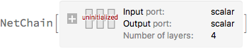
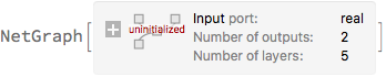
net = NetChain[
  {LinearLayer[nUnits], ElementwiseLayer[activation], DropoutLayer[pdrop], 
   LinearLayer[]},
  "Input" -> "Scalar",
  "Output" -> "Scalar"
  ]

Train the network:

trainedNet = NetTrain[
  net,
  <|"Input" -> exampleData[[All, 1]], "Output" -> exampleData[[All, 2]]|>,
  LossFunction -> MeanSquaredLossLayer[],
  Method -> {"ADAM", "L2Regularization" -> λ2}
  ]

This function takes a trained net and samples it multiple times with the dropout layers active (using NetEvaluationMode -> "Train"). It then constructs a timeseries object of the - 1, 0 and + 1 sigma bands of the predictions.

sampleNet[net : (_NetChain | _NetGraph), xvalues_List, 
  sampleNumber_Integer?Positive, {lengthScale_, l2reg_, prob_, 
   nExample_}] := TimeSeries[
  Map[
   With[{
      mean = Mean[#],
      stdv = 
       Sqrt[Variance[#] + (2 l2reg nExample)/(lengthScale^2 (1 - 
              prob))]
      },
     mean + stdv*{-1, 0, 1}
     ] &,
   Transpose@
    Select[Table[
      net[xvalues, NetEvaluationMode -> "Train"], {i, sampleNumber}], 
     ListQ]],
  {xvalues},
  ValueDimensions -> 3
  ]

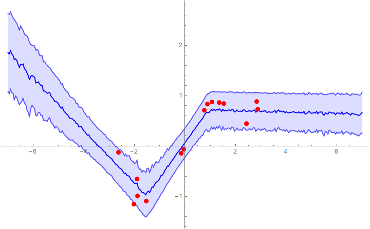
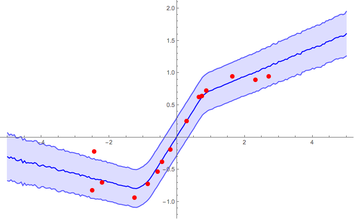
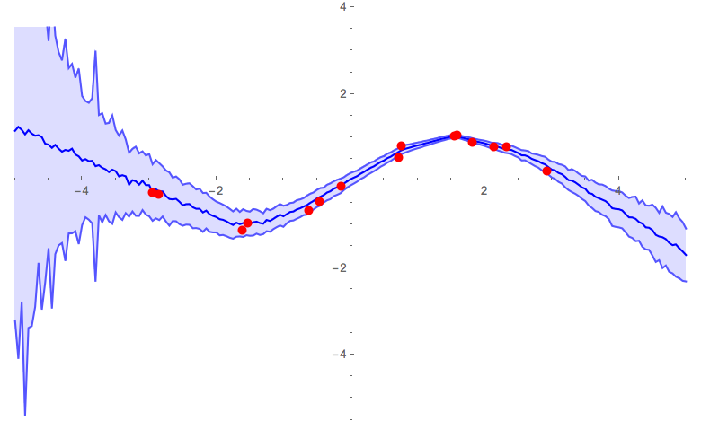
Now we can plot the predictions with 1σ error bands. The prior l=2 seems to work reasonably well, though in real applications you'd need to calibrate it with a validation set (just like Subscript[λ, 2] and p).

l = 2;
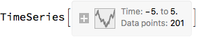
samples = sampleNet[trainedNet, Range[-5, 5, 0.05], 
  200, {l, λ2, pdrop, Length[exampleData]}]
Show[
 ListPlot[
  samples,
  Joined -> True,
  Filling -> {1 -> {2}, 3 -> {2}},
  PlotStyle -> {Lighter[Blue], Blue, Lighter[Blue]}
  ],
 ListPlot[exampleData, PlotStyle -> Red],
 ImageSize -> 600,
 PlotRange -> All
 ]

Heteroscedastic regression

exampleData = Table[(*initialise training data*){x, Sin[x]} + RandomVariate[NormalDistribution[0, .15]],
     {x, RandomVariate[UniformDistribution[{-3, 3}], 15]}];
ListPlot[exampleData]

In heteroscedastic regression we let the neural net try and find the noise level for itself (see section 4.6 in the PhD thesis by Yarin Gal linked at the top of the notebook). This means that the regression network outputs 2 numbers instead of 1: a mean and a standard deviation. However, since the output of the network is a real number, we interpret it as the log of the precision logτ = Log[τ] = Log[1/σ^2]:

λ2 = 0.01;
pdrop = 0.1;
nUnits = 200;
activation = Ramp;
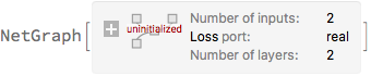
regressionNet = NetGraph[
  {LinearLayer[nUnits], ElementwiseLayer[activation], DropoutLayer[pdrop], 
   LinearLayer[], LinearLayer[]},
  {
   NetPort["Input"] -> 1 -> 2 -> 3,
   3 -> 4 -> NetPort["Mean"],
   3 -> 5 -> NetPort["LogPrecision"]
   },
  "Input" -> "Real",
  "Mean" -> "Real",
  "LogPrecision" -> "Real"
  ]

Next, instead of using a MeanSquaredLossLayer to train the network, we minimise the negative log-likelihood of the observed data. Again, we replace σ with the log of the precision and we multiplying by 2 to be in agreement with the convention of MeanSquaredLossLayer.

FullSimplify[-2*LogLikelihood[NormalDistribution[μ, σ], {yobs}] /. σ -> 1/Sqrt[Exp[logτ]], 
      Assumptions -> logτ \[Element] Reals]

Discarding the constant term gives us the following loss which we will incorporate into the net:

loss = Function[{y, mean, logPrecision},
   (y - mean)^2*Exp[logPrecision] - logPrecision
   ];
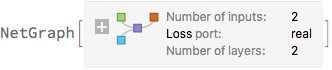
net = NetGraph[<|
   "reg" -> regressionNet,
   "negLoglikelihood" -> ThreadingLayer[loss]
   |>,
  {
   NetPort["x"] -> "reg",
   {NetPort["y"], NetPort[{"reg", "Mean"}], 
     NetPort[{"reg", "LogPrecision"}]} -> "negLoglikelihood" -> NetPort["Loss"]
   },
  "y" -> "Real",
  "Loss" -> "Real"
  ]

trainedNet = NetTrain[
  net,
  <|"x" -> exampleData[[All, 1]], "y" -> exampleData[[All, 2]]|>,
  LossFunction -> "Loss",
  Method -> {"ADAM", "L2Regularization" -> \[Lambda]2}
  ]

Again, the predictions are sampled multiple times. The predictive variance is now the sum of the variance of the predicted mean + mean of the predicted variance. The priors no longer influence the variance directly, but only through the network training. Note that we need to use NetExtract to get the regression net out of the trained net.

sampleNetHetero[net : (_NetChain | _NetGraph), xvalues_List, 
   sampleNumber_Integer?Positive] :=

  With[{regressionNet = NetExtract[net, "reg"]},
   TimeSeries[
    With[{
      samples = 
       Select[Table[
         regressionNet[xvalues, NetEvaluationMode -> "Train"], {i, 
          sampleNumber}], AssociationQ]
      },
     With[{
       mean = Mean[samples[[All, "Mean"]]],
       stdv = 
        Sqrt[Variance[samples[[All, "Mean"]]] + 
          Mean[Exp[-samples[[All, "LogPrecision"]]]]]
       },
      Transpose[{mean - stdv, mean, mean + stdv}]
      ]
     ],
    {xvalues},
    ValueDimensions -> 3
    ]
   ];

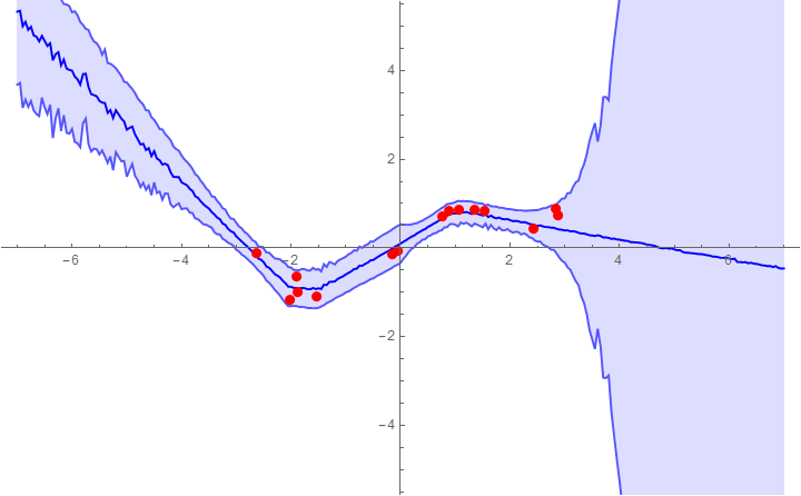
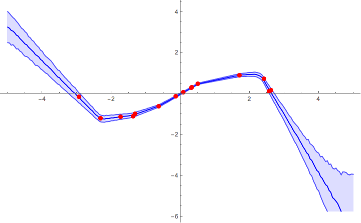
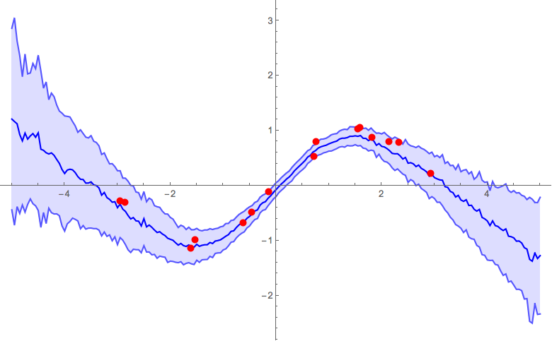
Now we can plot the predictions with 1σ error bands:

samples = sampleNetHetero[trainedNet, Range[-5, 5, 0.05], 200]
Show[
 ListPlot[
  samples,
  Joined -> True,
  Filling -> {1 -> {2}, 3 -> {2}},
  PlotStyle -> {Lighter[Blue], Blue, Lighter[Blue]}
  ],
 ListPlot[exampleData, PlotStyle -> Red],
 ImageSize -> 600,
 PlotRange -> All
 ]

Implementation of a loss function (from comments)

The following code shows how to implement the loss function described in the paper Dropout Inference in Bayesian Neural Networks with Alpha-divergences by Li and Gal: https://arxiv.org/pdf/1703.02914.pdf

In this paper, the authors propose a modified loss function α for a stochastic neural network (e.g., a network that uses dropout layers). During training, the training inputs Subscript[x, n] (with 1<=n<= N indexing the training examples) are fed through the network K times to sample the outputs Subsuperscript[Overscript[y, ~], n, k] and compared to the training outputs Subscript[y, n]. Given a particular standard loss function l (e.g., mean square error, negative loglikelihood, cross entropy) and regularisation function Subscript[L, 2] for the weights λ, the modified loss function L is given as:

The parameter α is the divergence parameter which can be tuned 0<α<=1

As can be seen, we need to sample the network several times during training. We can accomplish this with NetMapOperator. As a simple example, suppose we want to apply a dropout layer K=10 times to the same input. To do this, we duplicate the input and then wrap a NetMapOperatore around the dropout layer and map it over the duplicated input:

input = Range[5];
duplicatedInput = ConstantArray[input, 10];
NetMapOperator[
  DropoutLayer[0.5]
  ][duplicatedInput, NetEvaluationMode -> "Train"]

Let's implement this loss function for a simple regression example. First generate some example data:

exampleData = 
  Table[{x, Sin[x] + RandomVariate[NormalDistribution[0, .15]]}, {x, 
    RandomVariate[UniformDistribution[{-3, 3}], 15]}];
ListPlot[exampleData]

Next, define a net that will try to fit the data points with a normal distribution. The output of the net is a length-2 vector with the mean and the log-precision logτ = Log[τ] = Log[1/σ^2]:

alpha = 0.5;
pdrop = 0.5;
units = 200;
activation = Ramp;
λ2 = 0.001; (*L2 regularisation coefficient*)

k = 25; (* number of samples of the network for calculating the loss*)

regnet = NetInitialize@NetChain[{
     LinearLayer[units],
     ElementwiseLayer[activation],
     DropoutLayer[pdrop],
     LinearLayer[]
     },
    "Input" -> "Real",
    "Output" -> {2}
    ];

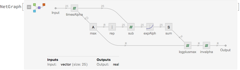
We will also need a network element to calculate the log-sum-exp operator that aggregates the losses of the different samples of the regression network. We implement the log-sum-exp in the following way (i.e., by factorising out the largest term before feeding the vector into the Exp operator) to make it more numerically stable:

logsumexp[alpha_] := 
  NetGraph[<|
    "timesAlpha" -> ElementwiseLayer[Function[-alpha #]],
    "max" -> AggregationLayer[Max, 1],
    "rep" -> ReplicateLayer[k],
    "sub" -> ThreadingLayer[Subtract],
    "expAlph" -> ElementwiseLayer[Exp],
    "sum" -> SummationLayer[],
    "logplusmax" -> ThreadingLayer[Function[{sum, max}, Log[sum] + max]],
    "invalpha" -> ElementwiseLayer[-(1/alpha) # &]
    |>,
   {
    NetPort["Input"] -> "timesAlpha",
    "timesAlpha" -> "max" -> "rep",
    {"timesAlpha", "rep"} -> "sub" -> "expAlph" -> "sum" ,
    {"sum", "max"} -> "logplusmax" -> "invalpha"
    },
   "Input" -> {k}
   ];
logsumexp[alpha]

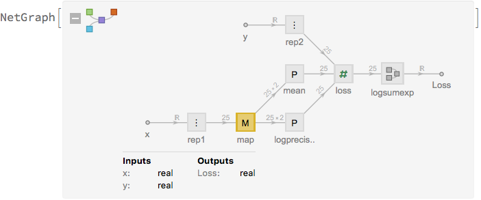
Define the network that will be used for training:

net[alpha_] := 
 NetGraph[<|
   "rep1" -> ReplicateLayer[k],(* 
   replicate the inputs and outputs of the network *)

   "rep2" -> ReplicateLayer[k],
   "map" -> NetMapOperator[regnet],
   "mean" -> PartLayer[{All, 1}],
   "logprecision" -> PartLayer[{All, 2}],
   "loss" -> 
    ThreadingLayer[
     Function[{mean, logprecision, y}, (mean - y)^2*Exp[logprecision] - 
       logprecision]],
   "logsumexp" -> logsumexp[alpha]
   |>,
  {
   NetPort["x"] -> "rep1" -> "map",
   "map" -> "mean",
   "map" -> "logprecision",
   NetPort["y"] -> "rep2",
   {"mean", "logprecision", "rep2"} -> "loss" -> "logsumexp" -> NetPort["Loss"]
   },
  "x" -> "Real",
  "y" -> "Real"
  ]
net[alpha]

and train it:

alpha = 0.1;
trainedNet = NetTrain[
net[alpha],
<|"x" -> exampleData[[All, 1]], "y" -> exampleData[[All, 2]]|>,
LossFunction -> "Loss",
Method -> {"ADAM", "L2Regularization" -> λ2},
TargetDevice -> "CPU",
TimeGoal -> 60
];

This function helps to sample the trained net several times to get a measure of the predictive mean and standard deviation:

sampleNetAlpha[net : (_NetChain | _NetGraph), xvalues_List, 
nSamples_Integer?Positive] := 
With[{regnet = NetExtract[net, {"map", "Net"}]},
 TimeSeries[
   Map[
    With[{
      mean = Mean[#[[All, 1]]],
      stdv = Sqrt[Variance[#[[All, 1]]] + Mean[Exp[-#[[All, 2]]]]]
    },
      mean + stdv*{-1, 0, 1}
    ] &,
    Transpose @ Select[
      Table[
        regnet[xvalues, NetEvaluationMode -> "Train"],
        {i, nSamples}
      ], ListQ]],
   {xvalues},
   ValueDimensions -> 3
  ]
];

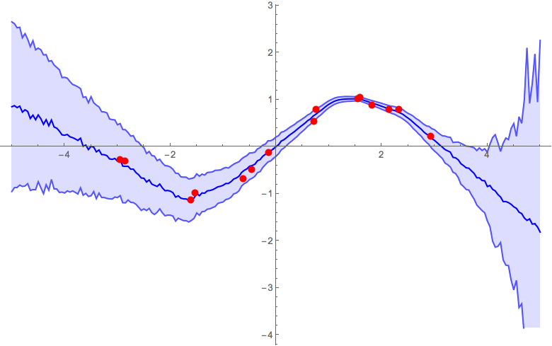
samples = sampleNetAlpha[trainedNet, Range[-5, 5, 0.05], 200];

Show[
 ListPlot[
  samples,
  Joined -> True,
  Filling -> {1 -> {2}, 3 -> {2}},
  PlotStyle -> {Lighter[Blue], Blue, Lighter[Blue]}
  ],
 ListPlot[exampleData, PlotStyle -> Red],
 ImageSize -> 600,
 PlotRange -> All
 ]

Ultimately, you'd need to do some validation tests to calibrate the parameters of your model. To give a feel of how the α parameter influences the result, below are some figures from previous runs with different α parameters. The other parameters that were used were: pdrop = 0.5; units = 200; activation = Ramp; λ2 = 0.001; k = 25;

α = 0.1

α = 0.5

α = 1

Interactive example

Below is a dynamic example (inspired by the link above) of a network that is continuously retrained on the data. You can edit the points by dragging the locators and delete points by alt-clicking.

DynamicModule[{
  exampleData,
  net ,
  prob = 0.2,
  \[Lambda] = 0.01,
  rounds = 10,
  sampleNumber = 100,
  samples,
  l = 2,
  nlayers = 300,
  activation = Ramp,
  init,
  sampleNet,
  xmin = -5,
  xmax = 5,
  ymin = -2,
  ymax = 2
  },
 exampleData = Table[ (*initialise training data *)
   {x, Sin[x]} + RandomVariate[NormalDistribution[0, .15]],
   {x, RandomVariate[UniformDistribution[{-3, 3}], 15]}
   ];

Function to sample the noisy net multiple times and calculate mean + stdev

 sampleNet[net_NetChain, xvalues_List, sampleNumber_Integer?Positive] := 
  PreemptProtect[
   TimeSeries[
    Map[
     With[{
        mean = Mean[#],
        stdv = Sqrt[Variance[#] + (2 \[Lambda] Length[exampleData])/(l^2 (1 - prob))]
        },
       mean + stdv*{-1, 0, 1}
       ] &,
     Transpose@Select[
       Table[
        net[xvalues, NetEvaluationMode -> "Train"],
        {i, sampleNumber}
        ],
       ListQ
       ]
     ],
    {xvalues},
    ValueDimensions -> 3
    ]
   ];

Network initialisation function. Necessary when one of the network parameters is changed.

 init[] := PreemptProtect[
   net = NetInitialize@NetChain[
      {
       LinearLayer[nlayers],
       ElementwiseLayer[activation],
       DropoutLayer[prob],
       1
       },
      "Input" -> "Scalar",
      "Output" -> "Scalar"
      ]
   ];
 init[];
 samples = sampleNet[net, N@Subdivide[xmin, xmax, 100], sampleNumber];

 DynamicWrapper[
   Grid[{
    (* Controls *)
    {
     Labeled[Manipulator[Dynamic[l], {0.01, 10}], 
      Tooltip["l", "GP prior length scale"], Right],
     Labeled[Manipulator[Dynamic[\[Lambda]], {0.0001, 0.1}], 
      Tooltip["\[Lambda]", "L2 regularisation coefficient"], Right]
     },
    {
     Labeled[Manipulator[Dynamic[sampleNumber], {10, 500, 1}], "# samples", 
      Right],
     SpanFromLeft
     },
    {
     Labeled[Manipulator[Dynamic[prob], {0, 0.95}, ContinuousAction -> False], 
      Tooltip["p", "Dropout probability"], Right],
     Labeled[
      Manipulator[Dynamic[nlayers], {20, 500, 1}, ContinuousAction -> False], 
      "# layers", Right]
     },
    {
     Labeled[
      PopupMenu[
       Dynamic[activation],
       {
        Ramp, Tanh, ArcTan, LogisticSigmoid, "ExponentialLinearUnit", 
        "ScaledExponentialLinearUnit",
        "SoftSign", "SoftPlus", "HardTanh", "HardSigmoid"
        },
       ContinuousAction -> False
       ],
      "Activation function"
      ,
      Right
      ],
     (* This resets the network if one of the network parameters changes *)
     DynamicWrapper[
      "",
      init[],
      SynchronousUpdating -> False,
      TrackedSymbols :> {activation, prob, nlayers}
      ]
     },

    (* Main contents *)
    {
     Labeled[
      LocatorPane[
       Dynamic[exampleData],
       Dynamic[
        Show[
         ListPlot[exampleData, PlotStyle -> Red],
         ListPlot[
          samples,
          Joined -> True,
          Filling -> {1 -> {2}, 3 -> {2}},
          PlotStyle -> {Lighter[Blue], Blue, Lighter[Blue]}
          ],
         ImageSize -> 600,
         PlotRange -> {{xmin, xmax}, {ymin, ymax}}
         ],
        TrackedSymbols :> {samples, exampleData}
        ],
        ContinuousAction -> False,
        LocatorAutoCreate -> All
       ],
      "1 \[Sigma] error bands (\[AltKey] + click to delete points)",
      Top
      ],
     SpanFromLeft
     }
    },
   BaseStyle -> "Text",
   Alignment -> Left
   ],

  (* Continuously retrain the net on the current examples and resample the network *)
  net = Quiet@With[{
      new = NetTrain[
        net,
        <|
         "Input" -> exampleData[[All, 1]],
         "Output" -> exampleData[[All, 2]]
         |>,
        LossFunction -> MeanSquaredLossLayer[],
        Method -> {"ADAM", "L2Regularization" -> \[Lambda], "LearningRate" -> 0.005},
        MaxTrainingRounds -> rounds,
        TrainingProgressReporting -> None
        ]
      },
     If[ Head[new] === NetChain, new, net]
     ];
  samples = sampleNet[net, N@Subdivide[xmin, xmax, 50], sampleNumber],
  SynchronousUpdating -> False
  ]
 ]