My WSS project is to study packing of Bidisperse circles, i.e., circles of 2 different radii. To do so, I implemented the Lubachevsky-Stillinger algorithm with an Event Driven approach, based on the algorithmic details here and here, and the C++ implementation here.
As for a heuristic algorithmic description, check out this gif:
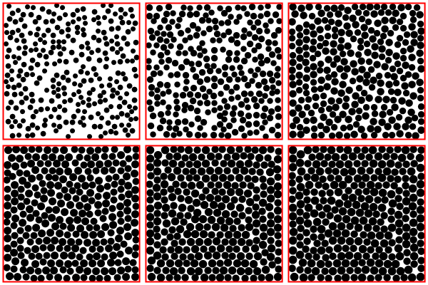
The disks are randomly initialized, and grow with time while colliding and bouncing around. Collisions are processed, new events are computed, and the simulation progresses until jamming (or a event error is flagged and the simulation aborts).
As for the implementation, I segmented it into 9 sections: Constraints, Initialization, Cell Method, Augmented MinHeap, Collisions, Transfers, Procedure, Visualization and Analysis. Each section has its own functions and description (43 functions total!), and I'll try to explain some of them here (I won't comment on Constraints because they are quite straightforward, nor the MinHeap, because it will get its own post).
Initialization
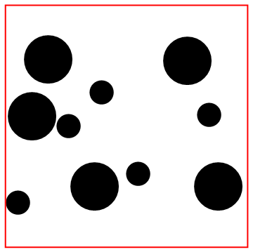
Here is where the initial radii, positions and velocities are defined. The initial positions need to satisfy the constraint functions, and to place another circle entails not overlapping any of the previously input circles, nor the square boundary. The function to do so is createDisk, below. It randomly tries circle coordinates, given a partial list of coordinates (circles) and a full list of radii (radii) which define the constraints.
createDisk[circles_List,radii_List, size_]:=Module[
{cnumber=circles//Length, position, riffled, count=0, insert=False, rc, r},

(*splice radii list, select next radius, riffle coordinates and radii for constraint functions*)
rc=radii[[;;cnumber]]; r=radii[[cnumber+1]]; riffled=Riffle[circles,rc]//Partition[#, 2]&;

(*testing loop*)
While[
(*stop when inserted or overcount*)
And[count<200, !insert ],

    (*randomly try next coordinate*)
    position=RandomReal[{0, size}, 2];

    (*if doesn't overlap border or overlap anyother circle*)
    If[And[
    borderC[position,r],
    And@@(overlapC[{position, r}, #]&/@riffled)
    ], insert=True];
count=count+1;
];
If[count==200, Print["fail"]];

position
]
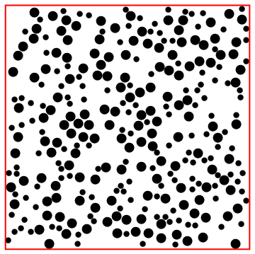
Nested application of createDisk.
Cell Method
Eventually, we will need to calculate the next collision time for some particle i . The easiest way to do so would be to calculate the times for all particles and take the minimum, but that would be computationally expensive for many body systems. Instead, I implemented the Cell Method, essentially segmenting the space into a grid, and placing each particle into bins (stored with a Matrix/Association pair). Now, instead of iterating over all particles to find the minimum collision time, just look at the particles in the neighboring bins. The functions below are 2 of the most important for this method: nearestCells and updateCell.
nearestCells
nearestCells takes a list of coordinates, number of rows and size and returns a matrix (rows, rows) of lists, where cellMatrix[[i, j]] stores the particle indices in that bin.
nearestCells[coordinates_, nrows_, size_]:= Module[
{nf=Nearest[coordinates->Range@Length@coordinates, DistanceFunction->ChessboardDistance]},
nf[binCenters[nrows, size], {Infinity, size/(2 nrows)}]
]
Where binCenters[nrows, size] returns a list of grid center coordinates. The visual representation: 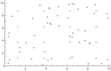
updateCell
As the disks move around, inevitably they will transfer between bins, and the correspondent cellMatrix (result of function above) and cellA (association mapping particle index to bin index pair) have to be updated. updateCell does exactly that:
updateCell[i_, newcell_] := Module[{currentk, currentj, oldk, oldj},
  (*initialize variables*)
  {currentk, currentj} = newcell;
  {oldk, oldj} = cellA[i];
  (*delete and reinsert element from cellMat*)
  cellMatrix[[oldk, oldj]] = Select[cellMatrix[[oldk, oldj]], # != i &]
  AppendTo[cellMatrix[[currentk, currentj]], i];
  (*reset element in association*)
  cellA[i] = {currentk, currentj};
  ]
Collisions
Here is where I implemented all collision-related functions: calculateCollision, predictCollision, findNextCollision, collisionCheck and processCollision. The first 3 are related to calculating the next collision for particle i, the 4^th enforces the collision is valid and symmetric (if i collides with j, j has to collide with i) and the last processes a collision event, through conservation of momentum. Here, events are parametrized by triples: {te, i, p}: te is the time of the event, i is the particle index, and p_Integer the event partner: if 0 < p < N+1, the event is a collision with particle p. Take a look at the 2 most important of them:
calculateCollision
This function calculates the collision time, if it exists (else, infinity). Additionally, this function aborts the program if there is considerable overlap between particles, and prints an error statement.
calculateCollision[i_, j_]:= Module[
{nRi, nRj, d, \[Sigma], \[CapitalDelta]R, \[CapitalDelta]V, A, B, C, t},
(*sets positions and radii to current time*)
nRi=positions[[i]]+(gtime-lastupdates[[i]])velocities[[i]];
nRj=positions[[j]]+(gtime-lastupdates[[j]])velocities[[j]];
\[Sigma]=(radii[[i]]+radii[[j]])^2;

(*define helper variables*)
\[CapitalDelta]R=nRi-nRj;
\[CapitalDelta]V=velocities[[i]]-velocities[[j]];
A=\[CapitalDelta]V.\[CapitalDelta]V-rate^2 \[Sigma];
B=\[CapitalDelta]V.\[CapitalDelta]R-rate(1+rate gtime)\[Sigma];
C=\[CapitalDelta]R.\[CapitalDelta]R-\[Sigma] (1+rate gtime)^2;
d=B^2-A C;

(*debugging tests*)
If[C<-10^(-2)(radii[[i]]+radii[[j]])(1+gtime rate), Print["After ", totalevents, " events, overlap."]; Abort[]];

(*calculate time*)
Which[
    C <-10^(-4)(radii[[i]]+radii[[j]])(1+gtime rate) && B < 0, Print["spheres are already overlapping ", C]; Infinity,

     d <= 0, Infinity,

    True, -(B+Sqrt[d])/(A)
    ]
]
collisionCheck
collisionCheck enforces collisions are symmetric, as well as updating p's event partner's events if necessary (see Procedure section for further details):
collisionCheck[collision_] := Module[
  {tc, i, j, symcol, k, n = nextevents // Length, ek},
  {tc, i, j} = collision;
  symcol = {tc, j, i};
  k = nextevents[[j]][[3]];
  (*j cannot have event before colliding with i*)
  If[tc > nextevents[[j]][[1]], Print["big mistake"]; Abort[]];

  (*if j's next event was collision, give k a check*)
  If[(k <= n) && (k != i) && (k >= 1),
   ek = nextevents[[k]];
   nextevents[[k]] = {ek[[1]], k, Infinity};];

  (*set symmetric collision as j's next event*)
  nextevents[[j]] = symcol;
  (*update Heap*)
  decreaseKey[j, tc];
  ]
Ignore the heap stuff for now, I'll explain in a bit.
Transfers
This section is related specifically to transfers: events corresponding to movement between cell walls. Each transfer event can be parametrized using the same triples, now, with N < p < N+5, where p-N indicates the specific cell wall: 1 for the right wall, 2 for the left, 3 for the top, 4 for the bottom. There are 2 functions in this section: findNextTransfer and processTransfer. The second is quite straightforward, and is basically a set of Which cases and updateCell calls. findNextTransfer, however, is just slightly more elaborated.
findNextTransfer
This function is also a set of Which cases, for each direction (1,2, 3 or 4), now considering radii growth if colliding with a hard boundary. See below:
findNextTransfer[i_]:= Module[
{r, rx, ry, vx, vy, wallindex, binindex, bincenter, step=size/nrows, times=Table[Infinity, {4}]},

(*set positions, set velocities, set radius*)
r = radii[[i]];
{rx, ry} = positions[[i]] + velocities[[i]](gtime-lastupdates[[i]]);
{vx, vy} = velocities[[i]];

(*obtain bin position*)
binindex = cellA[i];
bincenter = step(binindex - {1,1}/2);

(*consider x axis*)
Which[
    vx>0 && binindex[[1]]!=nrows,
       times[[1]]=(bincenter[[1]]+step/2-rx)/vx;,
    vx >0 && binindex[[1]] == nrows,
       times[[1]]=(bincenter[[1]]+step/2-rx-r(1 + gtime rate))/(vx+rate radii[[i]]);,
    vx<0 && binindex[[1]]!=1,
       times[[2]]=(bincenter[[1]]-step/2-rx)/vx;,
    vx <0 && binindex[[1]]==1,
       times[[2]]=(bincenter[[1]]-step/2-rx+r(1+gtime rate))/(vx-rate radii[[i]]);
];

(*consider y axis*)
Which[
    vy>0 && binindex[[2]]!=nrows,
       times[[3]]=(bincenter[[2]]+step/2-ry)/vy;,
    vy>0 && binindex[[2]] == nrows,
       times[[3]]=(bincenter[[2]]+step/2-ry-r(1+gtime rate))/(vy+rate radii[[i]]);,
    vy<0 && binindex[[2]]!=1,
       times[[4]]=(bincenter[[2]]-step/2-ry)/vy;,
    vy<0 && binindex[[2]]==1,
       times[[4]]=(bincenter[[2]]-step/2-ry+r(1+gtime rate))/(vy-rate radii[[i]]);
];
wallindex = Ordering[times][[1]];

(*debugging statement*)
If[!(And@@Positive@times), Print["negative time", times, binindex]; Print@borderC[{rx, ry}, r(1+gtime rate)]; Abort[]];

(*return event*)
{Min[times]+gtime, i, n+ wallindex}
]
Procedure
This section is where the previous sections come together. This section includes findNextEvent, ProcessEvent, and synchronize, as well as Process, which puts everything together. The first calls findNextTransfer and findNextCollision, and returns the event of lowest start time (with some complications). The second extracts the next event from the heap, processes the event, and calls findNextEvent on the particle in question and reinserts the new event into the heap.
Here, it is worth commenting on how the events are stored overall: a augmented min-heap stores tuples {te, i}, indicating the time te of particle i's next event. A list nextevents stores these events, where nextevents[[i]] is a event triple . This allows events to be inserted and the minimum time event obtained in a relatively fast time (O(log n) complexity for those operations, as well as lookup in O(1) with a association on top).
Now, let us take a look at these functions:
findNextEvent
In addition to the explanation above, findNextEvent has to account for and return an extra possibilities: In case particle i has outgrown it's own bin size, or will do so before the next collision or transfer, a p=-Infinity flag is set as the event partner to be processed later.
findNextEvent[i_] := Module[
{outgrowtime, step = size/(nrows), t, c, event,r},

r= radii[[i]];

outgrowtime = gtime+(step/2 - r(1+gtime rate))/(rate r);
If[outgrowtime < 0, outgrowtime = 0];

(*obtain transfer and collision events*)
t = findNextTransfer[i];
c = findNextCollision[i];

Which[

    (*outgrow event*)
    (outgrowtime < c[[1]]) && (outgrowtime < t[[1]]) && (nrows > 1),
       event = {outgrowtime, i, -Infinity};,

    (*next event is collision*)
    (c[[1]] < t[[1]]),
       collisionCheck[c];
       event = c;,

    (*next event is transfer*)
    (t[[1]] <= c[[1]]),
       event = t;
];

event
]
processEvent
This function processes exactly 1 event, outputting it from the heap and accessing it using nextevents. Then, the event is processed, and the next event for that particle is calculated, and inserted into the heap. Counters are set to sample data as the simulation progresses. If the event is a check (parametrized by p=Infinity), there is nothing to process and just obtain the next event. Moreover, if the event is an outgrowth (p=-Infinity), rescale the system, update the Cells (ChangeBins) and recommence the simulation.
processEvent := Module[ {te, i, j, nextevent, cevent},

(*increment counter, store data*)
nevents++;
If[Divisible[nevents, Ceiling[steps/20]], dataStore[]];

(*extract event from heap, initialize event variables*)
{te, i} = obtainMin[heap];
j = nextevents[[i]][[3]];
cevent = nextevents[[i]];

(*Divide into event cases*)
Which[
    (*event is a collision*)
    (j >= 1) && (j <= n),

       (*process collision*)
       ncollisions = ncollisions + 1;
       processCollision[{te, i, j}];

       (*make sure event was symmetric and check j*)
       If[ (nextevents[[j]][[3]] != i) || (nextevents[[j]][[1]] != gtime),
         Print["Events not symmetric", cevent, nextevents, gtime];
         Abort[],
         nextevents[[j]][[3]] = Infinity;
       ];

       (*set next event*)
       nextevent = findNextEvent[i];
       nextevents[[i]] = nextevent;
       increaseKey[i, nextevent[[1]]];

       If[te >= nextevent[[1]], Print["collision event time error"]];
    ,

    (*event is a transfer*)
    (j > n) && (j < n + 5),

       (*process transfer*)
       ntrans = ntrans + 1;
       processTransfer[{te, i, j}];

       (*set next event*)
       nextevent = findNextEvent[i];
       nextevents[[i]] = nextevent;
       increaseKey[i, nextevent[[1]]];

       If[te >= nextevent[[1]], Print["transfer event error", cevent, nextevent]; Abort[]];
    ,

    (*event is a check*)
    j == Infinity,

       (*process check*)
       nchecks = nchecks + 1;

       (*set next event*)
       nextevent = findNextEvent[i];
       nextevents[[i]] = nextevent;
       increaseKey[i, nextevent[[1]]];

       If[te > nextevent[[1]] && nextevent[[3]]!= -Infinity,
       Print["check event error", cevent, nextevent];
       ];
    ,

    (*disk outgrew cell, decrease nrows*)
    j == - Infinity,

       (*synchronize system*)
       gtime = te;
       synchronize[False];
       nrows = nrows - 1;

       (*need to resize system and update parameters*)
       changeBins[nrows];
       setInitialEvents[n];

       Process[steps];
    ];
];
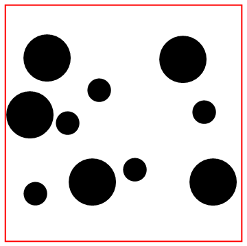
Look at the bottom particle colliding with the wall!
Visualization
Here, I built a visualization function to display circles of different radii using Riffle. A couple results have already been shown above.
displayParticles
displayParticles[positions_, radii_, size_]:= Module[
{rifflelist, border, borderg},
border = Line@{{0,0}, {0, size}, {size, size}, {size, 0}, {0 ,0}};
borderg =  Graphics[{Thick, Red, border}];
rifflelist = Riffle[positions, radii]//Partition[#, 2]&;
Show[Graphics[{Disk[#[[1]], #[[2]]]&/@rifflelist}], borderg]
]
Analysis
Finally, a couple functions to analyze the simulation results.
packingFraction
packingFraction := radii.radii Pi (1 + rate gtime)^2/size^2
dataStore
Appends position and current radii, for visualization purposes, as well as the current packing fraction.
dataStore:=(
AppendTo[pf, packingFraction];
    nestpositions = AppendTo[nestpositions, positions];
    nestradii = AppendTo[nestradii, radii];
)
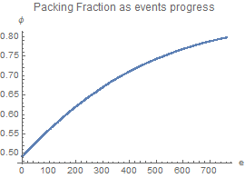
I attached my full implementation below, with a couple more simulations and plots, and additional documentation for the functions not explained above. There still are precision errors, and I still plan to add further analysis functions and simulations of different systems (different particle number, radii ratio and particle ratio). To optimize the pack, do play around a lot with the initialization constants (initial packing fraction, initial velocities and growth rate). If any optimizations are found, please send me them!
 Attachments: