Gerrymandering is a practice that has been under intense scrutiny, especially as of recent with the Supreme Court being forced to make decisions on a not well understood topic. In this post, I will offer an alternative to the redistricting process. By incorporating FIPS codes and data for each tract, I will use graph theory by exploring the capabilities of the FindGraphPartition function, dividing various states into compact and contiguous districts. I will then incorporate geometric data to combine the shape of each tract with the tract's respective location. I then compare my synthetic districts to real congressional districts.
My code will ultimately create synthetic districts like the one seen bellow. 
What is a FIPS Code
A FIPS code is used to identify US State, County, and Tract. An example of one is below.
12 345 678901
The First two numbers are the state number; the following two are county, and the last six are the tract number. A census tract is the smallest territorial entity that has publicly available population data, usually containing about 4000 people.
Functions
This code selects the takes the tracts of Texas.
texasTractQ[v_Integer] := Take[IntegerDigits[v, 10, 11], 2] === {4, 8}
This code tells if two adjacent FIPS codes are in the same state.
texasEdgeQ[UndirectedEdge[source_, sink_]] := And[texasTractQ[source], texasTractQ[sink]]
This code is crucial in later assigning edge weight. The code identifies whether the connection between two bordering tracts cross county lines.
sameStateDifferentCountyQ[u : UndirectedEdge[source_, sink_]] :=
 Module[{sourceDigits, sinkDigits},
  sourceDigits = IntegerDigits[source, 10, 11];
  sinkDigits = IntegerDigits[sink, 10, 11];
  And[Take[sourceDigits, 2] == Take[sinkDigits, 2],
   Take[sourceDigits, {3, 5}] != Take[sinkDigits, {3, 5}]]
  ]
Create Edges
This code creates tract edges for all of the United States and then Texas. Each tract has an edge to its adjacent tract.
allEdges = Apply[UndirectedEdge, Rest@nlist, {1}]
texasEdges = Select[allEdges, texasEdgeQ];
Create Graphs
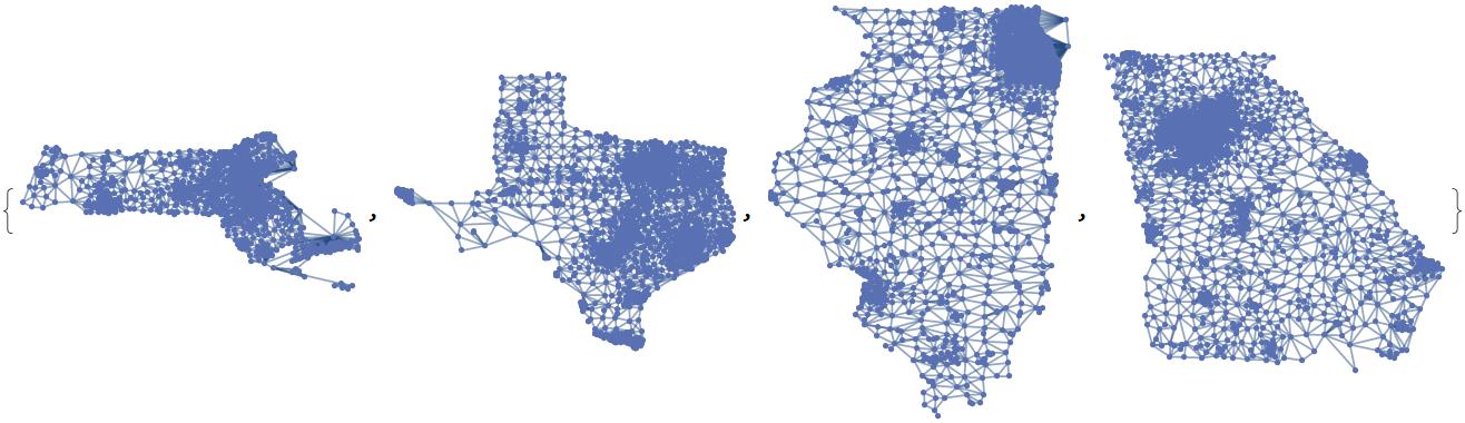
Here are graphs displaying states with each vertex being a tract and each edge being a connection between an adjacent tract. I will later use these graphs in partitioning.
texas = Graph[DeleteDuplicates[Sort /@ texasEdges]]
The same can be done for any other state.
illinois = Graph@DeleteDuplicates@Map[Sort, illinoisEdges]
Tract Data
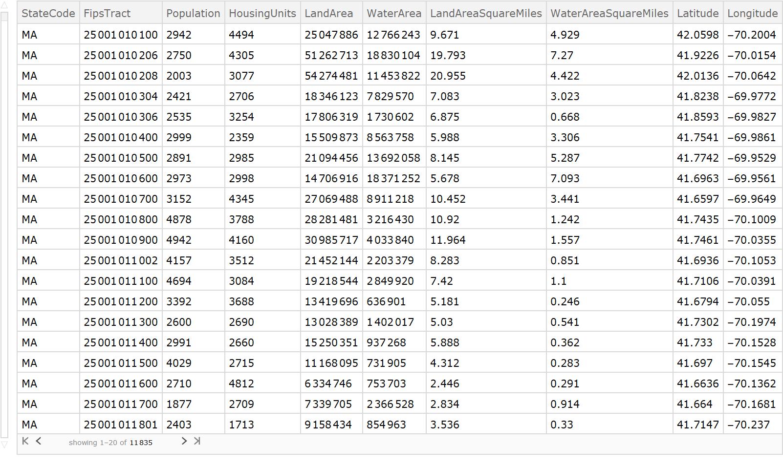
These graphs, however, are completely unrecognizable. To change that, I must get more data. This code creates a Dataset containing, among other things, the FIPS tract numbers and their respective population and geographic data. It is necessary for assigning vertex and edge weights later in my project.
headers = {"StateCode", "FipsTract", "Population", "HousingUnits",
   "LandArea", "WaterArea", "LandAreaSquareMiles",
   "WaterAreaSquareMiles", "Latitude", "Longitude"};
massTexasIllGaDS =
 Dataset[Map[AssociationThread[headers, #] &,
   Join[Rest@massTractTSV, Rest@texasTractTSV, Rest@illTractTSV,
    Rest@georgiaTractTSV]]]
Population Associations
By creating an association between FIPS code and population, my FindGraphPartitioning code will "snip" or cut each district and tracts with lower populations. In general, this allows each districting to have higher populations near the center of the districts, in affect, creating more realistic districts.
In[40]:= populationAssociation =
 Normal@Query[Association, #FipsTract -> #Population &][massTexasIllGaDS]
Geographic Associations and Creation of Alternative Graph Embeddings
Before dividing all states into districts, I will utilize the association between each FIPS tract and its respective coordinates to create a geographic view of each state.
geographicEmbedding[g_Graph, f_] :=
SetProperty[g, VertexCoordinates -> Map[f, VertexList[g]] ]

geoAssociation =
  Normal@Query[Association, #FipsTract -> {#Longitude, #Latitude} &][
    massTexasIllGaDS], 10]
I here define the geological graph of each state with the nodes at their respective latitude and longitude coordinates.
{massachusettsGeo, texasGeo, illinoisGeo, georgiaGeo} =
 Map[geographicEmbedding[#, geoAssociation] &, {massachusetts, texas,
   illinois, georgia}]
Discussion and Vocabulary
A district is a list of vertices. In our case, each vertex will be a tract. One can construct a subgraph that is "induced" by the vertices by making a graph that has all of the edges in the original graph that go between vertices in the district. If this sounds abstract, I have included an example below.
In[45]:= VertexList[dolphins]

Out[45]= {"Beak", "Beescratch", "Bumper", "CCL", "Cross", "DN16", \
"DN21", "DN63", "Double", "Feather", "Fish", "Five", "Fork", \
"Gallatin", "Grin", "Haecksel", "Hook", "Jet", "Jonah", "Knit", \
"Kringel", "MN105", "MN23", "MN60", "MN83", "Mus", "Notch", \
"Number1", "Oscar", "Patchback", "PL", "Quasi", "Ripplefluke", \
"Scabs", "Shmuddel", "SMN5", "SN100", "SN4", "SN63", "SN89", "SN9", \
"SN90", "SN96", "Stripes", "Thumper", "Topless", "TR120", "TR77", \
"TR82", "TR88", "TR99", "Trigger", "TSN103", "TSN83", "Upbang", \
"Vau", "Wave", "Web", "Whitetip", "Zap", "Zig", "Zipfel"}
A districting is a list of districts that should (when flattened) contain all of the vertices in the underlying graph. It is often called a partition of a graph. This means no vertex (dolphin, tract) should be in more than one district and every dolphin and tract is in one district. Another word for a district once the graph is disconnected is a "component".
Here is a districting of dolphins. Since all dolphins were created equal, the vertex weight for each dolphin will be one.
In[50]:= FindGraphPartition[dolphins, 3]
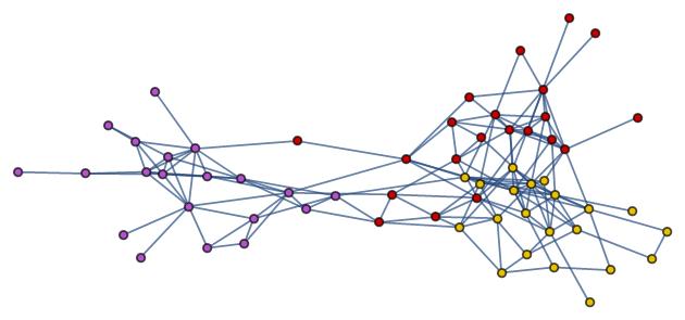
Partitioning Functions
Each subgraph is a district. This code uses polymorphism to make sure that all subgraphs are connected in a partitioning.
In[52]:= allConnectedQ[subgraphs : {___Graph}] :=
 And @@ Map[ConnectedGraphQ, subgraphs]

In[53]:= allConnectedQ[g_Graph, districting : List[__List]] :=
 allConnectedQ[Map[Subgraph[g, #] &, districting]]
I create a edge weight function that later allows assignments of edge weights based off if the edge crosses county borders. This uses the previously created sameStateDifferentCountyQ command.
In[54]:= countyBasedWeightingFunction[distributionInterCounty_,
  distributionIntraCounty_] :=
 If[sameStateDifferentCountyQ[#], RandomVariate[distributionInterCounty],
   RandomVariate[distributionIntraCounty]] &

In[55]:= Options[FindExactGraphPartitions] = {"VertexWeightFunction" -> (1 &),
  "EdgeWeightFunction" -> (1 &), "Wanted" -> 1, "MaxIters" -> 100,
  "Report" -> None}
FindGraphPartitions ultimately rests on the built in FindGraphPartition function, which in turn rests on the multi-level partitioning algorithm contained in software called METIS. Basically, what one does, is to collapse vertices (merge vertices into a kind of super-vertex) that are tightly connected and one keeps doing that until the graph is much smaller. Then, you can call other graph partitioning software algorithms (such as spectral methods) and partition the collapsed graph into the desired number of components (districts). Then, you uncollapse the graph and fiddle with local adjustments moving a few vertices from one component to another.
This line of code partitions each state into districts, with vertex weights being based off population and edge weights being lower if the edges cross county lines. The Option Values of Wanted and MaxIters allow one to later pick how many valid districtings they want and how many partitionings one will attempt. A partitioning is deemed successful in this code if the number of desired districts equals the number of created districts. Since the edge weights and vertex weights are assigned around a random distribution, each partitioning is different. In some failed partitionings, the number of partitions will exceed the number of desired partitions. I use the While command to allow one to enter the number of successful districts desired and the number of maximum attempt of FindGraphPartition with also using OptionValue. When a graph succesfully partitions into the number of desired districts, the value for found increases by one.
In[56]:= FindExactGraphPartitions[g_, rest___,
  OptionsPattern[FindExactGraphPartitions]] :=
 Module[{found = 0, tried = 0, g2, kc},
  While[Or[found < OptionValue["Wanted"], tried < OptionValue["MaxIters"]],
   (g2 = SetProperty[
      g, {VertexWeight ->
        Map[OptionValue["VertexWeightFunction"], VertexList[g]],
       EdgeWeight -> Map[OptionValue["EdgeWeightFunction"], EdgeList[g]]}];
    kc = FindGraphPartition[g2, rest];
     tried = tried + 1;
    If[allConnectedQ[g, kc], (Sow[kc]; found = found + 1;
      If[OptionValue["Report"] =!= None,
       Echo[StringTemplate["found success #`1` on try #`2`"][found, tried],
        "status"]];
      If[found >= OptionValue["Wanted"], Break[]]),
     If[OptionValue["Report"] === "Always",
      Echo[StringTemplate["failed on try #`1`"][tried], "status"]]])];
  Association["found" -> found, "tried" -> tried,
   "success rate" -> found/tried]
  ]
Metric Functions
- Rough equality of population in districts
In the code below, f should be a function that takes a district as an argument and returns its population. Alternatively, f can be an Association because Associations act like functions. Map[Total,{{f[402],f[401]},{f[304],f[309]}}]
The following code assesses population deviation in an attempt to assess how uniform each partitioned district's population is.
In[58]:= populationTotals[f_, districting : List[__List]] :=
  Map[Total, Map[f, districting, {2}]];

In[59]:= populationDeviation[l_List] := {-1, 1}.MinMax[l]/Mean[l]
This line of code is a metric I developed to assess compactness. Since each partition is not a geometric shape (yet), I will use this code as an intermediate tester for compactness. The lower the number, the more compact. 
In[63]:= compactnesses[g_, districting : List[__List]] :=
Map[compactness[g, #] &, districting]
Testing
Reap[kcutExact[stuff]] creates a list. The first element of the list containing an association. The second element of the list is a list which contains a single item, which is a list of districtings.
In[65]:= districtings[reapStructure : {a_Association, {ds_List}}] := ds

In[66]:= success[reapStructure : {a_Association, _}] := a
Once again, I begin with dolphins to make sure the code functions correctly. I see here that it took under twenty tries to find successful districtings of dolphins. The code will stop once the number of "Wanted" successful partitions is met, or once the number of partition attempts exceeds the "MaxIters" value.
    In[67]:= kceDolphins =
      Reap[FindExactGraphPartitions[dolphins, 4,
        "EdgeWeightFunction" -> (RandomVariate[NormalDistribution[1, 0.2]] &),
        "Wanted" -> 10, "MaxIters" -> 500, "Report" -> "Always"]];

status found success #1 on try #1

status found success #2 on try #2

status found success #3 on try #3

status failed on try #4

status found success #4 on try #5

status found success #5 on try #6

status failed on try #7

status found success #6 on try #8

status found success #7 on try #9

status found success #8 on try #10

status failed on try #11

status found success #9 on try #12

status found success #10 on try #13
The same is done for the other states
n[250]:= Short[Timing[
  kceMass = Reap[
     FindExactGraphPartitions[massachusetts, 9,
      "VertexWeightFunction" -> populationAssociation,
      "EdgeWeightFunction" ->
       countyBasedWeightingFunction[NormalDistribution[1, 0.2],
        NormalDistribution[1.5, 0.2]], "Wanted" -> 50, "MaxIters" -> 100,
      "Report" -> True]];]]
Due to the size of Texas and the desired 36 number of districts, a sharp increase from 9, the number of iterations to get districts correctly partitioned into the correct number of districts sharply increases. To conserve space, I will only show one succesfull partition. For the statistics later in the post, however, I use 200 successful partitions, creating 7200 valid districts.
In[407]:= kceTexas = Reap[FindExactGraphPartitions[texas, 36, "VertexWeightFunction" -> populationAssociation, "EdgeWeightFunction" -> countyBasedWeightingFunction[NormalDistribution[1, 0.2], NormalDistribution[1.5, 0.2]], "Wanted" -> 1, "MaxIters" -> 200, "Report" -> "Success"]];
status found success #1 on try #17
Visualization of Districting
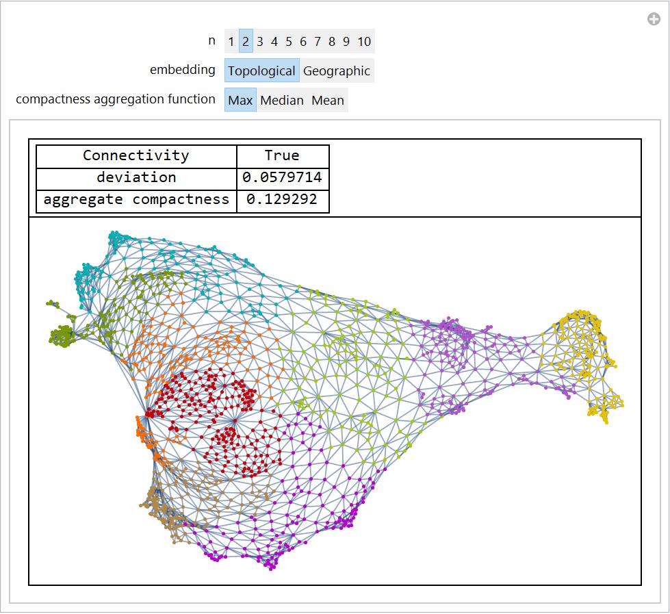
I created a manipulation tool to show successful partitions of each graph. One can select between successful partitions. Once again, I began with dolphins. This code incorporates previously defined algorithms that measure population deviation and compactness.
    manipulateFunction[g_Graph, kce_List ,
      n_Integer, populationAssociation_, acFunction_,
      opts : OptionsPattern[Graph]] :=
     Module[{districting, connectivity, population, deviation, cm,
       aggregateCompactness, visualization},
      districting = districtings[kce][[n]];
      connectivity = allConnectedQ[g, districting];
      population = populationTotals[populationAssociation, districting];
      deviation = populationDeviation[population];
      cm = N@compactnesses[g, districting];
      aggregateCompactness = acFunction[cm];
      visualization =
       HighlightGraph[g, districting, ImageSize -> 500, opts];
      Column[{Grid[{{"Connectivity", connectivity}, {"deviation",
           N@deviation}, {"aggregate compactness", aggregateCompactness}},
          Dividers -> All], visualization}, Dividers -> All]]

Manipulate[
manipulateFunction[dolphins, kceDolphins, n, 1 &, acFunction],
{n, Range[Length[districtings[kceDolphins]]],
ControlType -> SetterBar},
{{acFunction, Max, "compactness aggregation function"}, {Max, Median,
Mean}}]
Below are manipulate functions for selected states. The switch function was used to allow users to switch between a topological and geographic view. The deviation and compactness is given for each partition. Each color is one subgraph or district.
Manipulate[manipulateFunction[
    Switch[embedding, "Topological", massachusetts, "Geographic",
    massachusettsGeo], kceMass, n, populationAssociation, acFunction],
    {n, Range[Length[districtings[kceMass]]], ControlType -> SetterBar},
    {embedding, {"Topological", "Geographic"}},
    {{acFunction, Max, "compactness aggregation function"}, {Max, Median,
    Mean}}]
Edges that go through counties are once again given a lower weight. One can apply this code for any state. 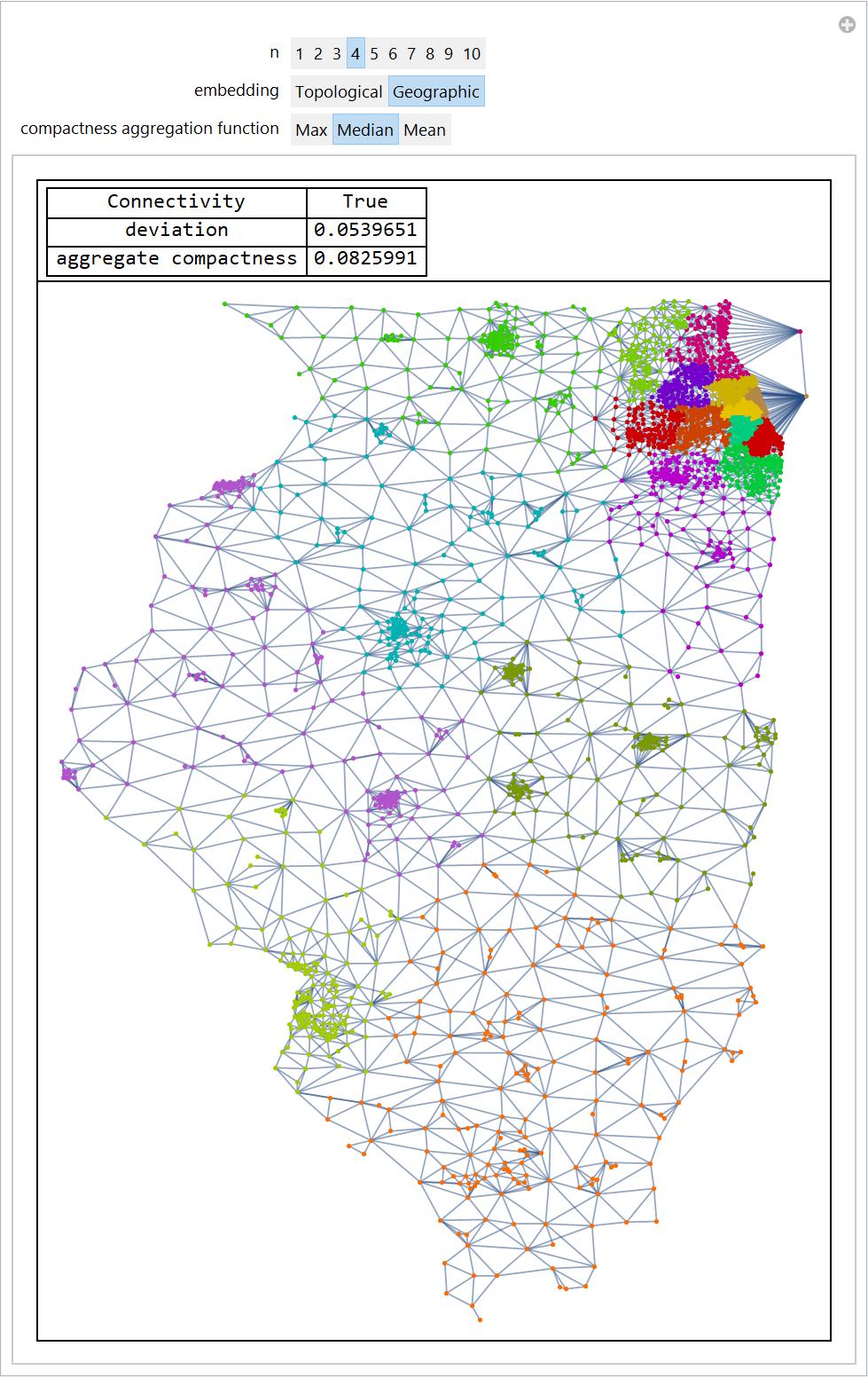
This code is a function that returns for every districting a list containing the districting's population deviation and its median aggregate compactness.
deviationCompactness[acFunction_] :=
 districting \[Function] {N@
    populationDeviation[
     populationTotals[populationAssociation, districting]],
   N@acFunction[compactnesses[massachusetts, districting]]}
medianDeviationCompactness = deviationCompactness[Median];
points = Map[medianDeviationCompactness, districtings[kceMass100]]
This code is a scatterplot that compares the relationship between population deviation and compactness. No strong correlation can be found between the two.
ListPlot[points,
 AxesLabel -> {"deviation", "aggregate (median) compactness"}]
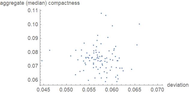
One could continue to use graph theory to compare compactness to population deviation, but I had a better idea.
Import and Association Creation For Tract Polygon Data
I import data here for the corresponding polygon shape for each census tract. The idea is to combine the existing shape of each tract onto each corresponding vertex in my partitioning of states. This allows me to geometrically assess the compactness of graphically partitioned states. The files were found on census.gov.
txshp = Import["C:\\Users\\alex2\\Downloads\\censusTractGeometry.wxf",
    "WXF"];
coloradoshp =
  Import["C:\\Users\\alex2\\Downloads\\censusTractGeometry08.wxf",
   "WXF"];
allTheTXTracts =
 Map[ToExpression,
  StringJoin @@@
   Thread[List[txshp[[4, 2, 1, 2]], txshp[[4, 2, 2, 2]],
     txshp[[4, 2, 3, 2]]]]
polygonTXAssociation =
  AssociationThread[allTheTXTracts, txshp[[2, 2]]];
Compactness Synthetic Districts
SyntheticDistrictArea is used to calculate the area of the polygons for each tract.
SyntheticDistrictArea[FipsTractToPolygonAssociation_,
  PolygonsForSyntheticDistrict_] :=
 Total[DeleteCases[
   Flatten[GeoArea[
     Lookup[FipsTractToPolygonAssociation,
      PolygonsForSyntheticDistrict]]], _Missing]]
This gives the smallest enclosing circle of any set of polygons. When using BoundingRegion with the specification of MinDisk, the code created a circle that was too big for many districts. This lowered my compactness score and was an unreliable measurement. GeoPositionXYZ was useful in representing positions in a Cartesian geocentric coordinate system. Credit goes to Chip Hurst for coming up with applying MinBall instead of just MinDisk to account for the curvature of the earth. This will be used as my denominator when calculating the compactness of my synthetic districts.
minGeoDisk[polygons_] :=
 Module[{pts, pts3D, sphere, minpts, rc, center, radius},
  pts = Cases[
    polygons /.
     GeoPosition[
       p_] :> (p /. {x_Real, y_} :> {y, x}), {_Real, _Real}, \[Infinity]];
  pts3D = GeoPositionXYZ[GeoPosition[Reverse[pts, {2}]]][[1]];
  sphere = Sphere @@ BoundingRegion[pts3D, "MinBall"];
  minpts = MinimalBy[DeleteDuplicates[pts3D], RegionDistance[sphere], 3];
  rc = RegionCentroid[
    RegionIntersection[Ball @@ sphere, InfinitePlane[minpts]]];
  center = Most /@ GeoPosition[GeoPositionXYZ[rc]];
  radius =
   UnitConvert[Quantity[EuclideanDistance[First[minpts], rc], "Meters"],
    "Miles"];
  GeoDisk[center, radius]
  ]

MinGeoDiskArea[FipsTractToPolygonAssociation_,
  PolygonsForSyntheticDistrict_] :=
 GeoArea[minGeoDisk[
   Lookup[FipsTractToPolygonAssociation, PolygonsForSyntheticDistrict]]]
Finally, the top two lines of code are combined to create one compactness measurement function.
CompactnessScore[FipsTractToPolygonAssociation_,
  PolygonsForSyntheticDistrict_] :=
 SyntheticDistrictArea[FipsTractToPolygonAssociation,
   PolygonsForSyntheticDistrict]/
  MinGeoDiskArea[FipsTractToPolygonAssociation, PolygonsForSyntheticDistrict]
Compactness Measurement For Real Districts
Using similar logic to the code above, this code uses calculates the minimum enclosing circular area (the denominator) for real districts. The numerator is simply a GeoArea calculation for the polygon form of a district.
minGeoDiskArea[polygons_] :=
 Module[{pts, pts3D, sphere, minpts, rc, center, radius},
  pts = Cases[
    polygons /.
     GeoPosition[
       p_] :> (p /. {x_Real, y_} :> {y, x}), {_Real, _Real}, \[Infinity]];
  pts3D = GeoPositionXYZ[GeoPosition[Reverse[pts, {2}]]][[1]];
  sphere = Sphere @@ BoundingRegion[pts3D, "MinBall"];
  minpts = MinimalBy[DeleteDuplicates[pts3D], RegionDistance[sphere], 3];
  rc = RegionCentroid[
    RegionIntersection[Ball @@ sphere, InfinitePlane[minpts]]];
  center = Most /@ GeoPosition[GeoPositionXYZ[rc]];
  radius =
   UnitConvert[Quantity[EuclideanDistance[First[minpts], rc], "Meters"],
    "Miles"];
  GeoArea[GeoDisk[center, radius]]]

CompactnessStateDistricts[statename_String] :=
 Flatten[GeoArea[
    Map[#["Polygon"] &,
     Flatten[Values[
       KeyTake[KeyDrop[
         GroupBy[EntityList[
           "USCongressionalDistrict"], #["USState"] &], {"DistrictOfColumbia",
           Missing["NotApplicable"], Missing["NotAvailable"]}],
        statename]]]]]/
   Map[minGeoDiskArea[#] &,
    Map[#["Polygon"] &,
     Flatten[Values[
       KeyTake[KeyDrop[
         GroupBy[EntityList[
           "USCongressionalDistrict"], #["USState"] &], {"DistrictOfColumbia",
           Missing["NotApplicable"], Missing["NotAvailable"]}],
        statename]]]]]]
Visualizing Synthetic Districts
I created the following manipulation tools in order to demonstrate the effectiveness of he incorporating graph partitioning code and geometric data for each node.
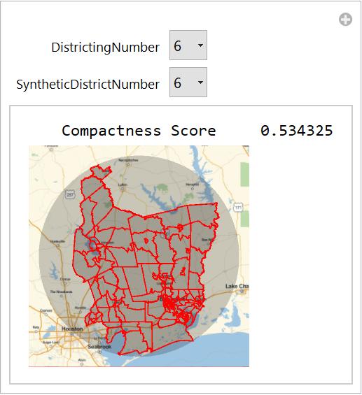
Texas Manipulate Tool
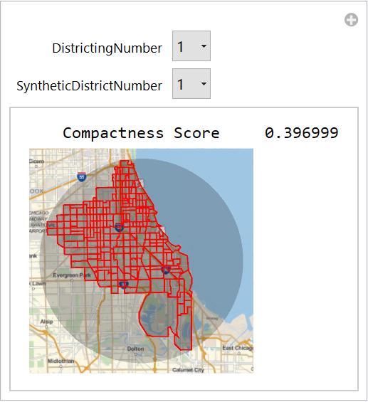
This code creates a manipulation tool that allows you to select from created fake districtings of Texas and their respective districts. The lower edge weights at the boundaries of counties creates partitionings of Texas that break districts closer to their county lines, creating more realistic districts. Every red polygon is one real tract with the enclosing area being my synthetic district.
Quiet@Manipulate[
  Grid[{{"Compactness Score",
     CompactnessScore[polygonTXAssociation,
      districtings[kceTexas][[DistrictingNumber]][[
       SyntheticDistrictNumber]]]}, {GeoGraphics[{minGeoDisk[
        Lookup[polygonTXAssociation,
         districtings[kceTexas][[DistrictingNumber]][[
          SyntheticDistrictNumber]]]], {EdgeForm[Red],
        Lookup[polygonTXAssociation,
         districtings[kceTexas][[DistrictingNumber]][[
          SyntheticDistrictNumber]]]}}]}}], {DistrictingNumber,
   Range[Length[districtings[kceTexas]]]}, {SyntheticDistrictNumber,
   Range[Length[
     districtings[kceTexas][[
      7]]]]}](*{DistrictingNumber,Range[Length[districtings[kceTexas]]\
]}*)
Illinois Manipulate Tool
Compactness Analysis and Visualizing
Using my CompactnessStateDistricts function, I get the compactness for real districts in the following states
texasdistrictcompactnessdata = CompactnessStateDistricts["Texas"];
syntheticdistrictcompactnessdataTexas =


Table[CompactnessScore[polygonTXAssociation,
districtings[kceTexas][[z]][[i]]], {z, 1, 200}, {i, 1, 36}];
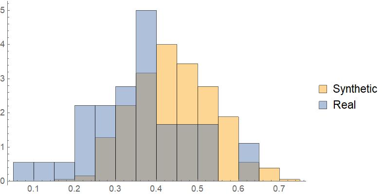
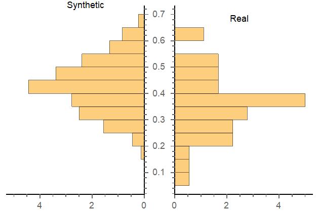
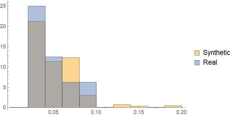
Here are some visualizations
Histogram[{txSyntheticCompactness,
  texasdistrictcompactnessdata}, Automatic, "PDF",
 ChartLegends -> {"Synthetic", "Real"}]
PairedHistogram[txSyntheticCompactness, texasdistrictcompactnessdata, \
Automatic, "PDF", ChartLabels -> {"Synthetic", "Real"}]
Statistical Testing
I took 36 draws from the synthetic distribution and computed the mean 10,000 times. There are 36 real congressional districts in Texas.
Short[meanSynthetic =
  Mean /@ RandomChoice[txSyntheticCompactness, {10000, 36}]]
I then found out the number of occasions on which the mean compactness in the real data is as large as the mean from the synthetic data.
In[152]:= Counts[
 Map[Mean[texasdistrictcompactnessdata] > # &, meanSynthetic]]
Out[152]= <|False -> 10000|>
Never! This is certainly very strong evidence that the real distribution does not come from the same process I used. Indeed, there may be more powerful statistical tests that would detect the falsity of the null hypothesis when the means comparison test would not do so. Here is another way of going about it.
In[308]:= LocationTest[txSyntheticCompactness,
 Mean@texasdistrictcompactnessdata, {"Sign", "TestConclusion"}]

Out[308]= {5.11282*10^-22,
 Row[{"The null hypothesis that ",
   Row[{"the ", "mean", " of the population is equal to ", 0.360349,
     " "}], "is rejected at the ", Row[{5, " percent level "}],
   Row[{"based on the ", "T", " test."}]}]}
Importing Racial Data
I import the following data with the purpose of later comparing racial distributions of my synthetic districts to real ones. All data comes directly from census.gov. I then created associations to calculate the percentage of white and African American people in each synthetic and real district.
Visualization for Analysis of Racial Distribution
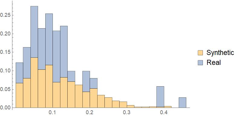
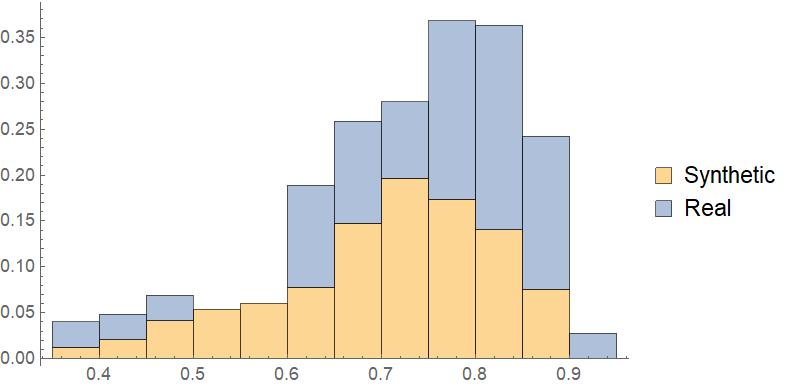
Histogram Representing The African American Percentage in both Real and Synthetic Districts for Texas
Histogram[{Flatten[
blackpopsforsyntheticdistricts/totalpopforsyntheticdistricting //
N], TexasDistrictBlackProportion}, Automatic, "Probability",
ChartLegends -> {"Synthetic", "Real"}, ChartLayout -> "Stacked"]
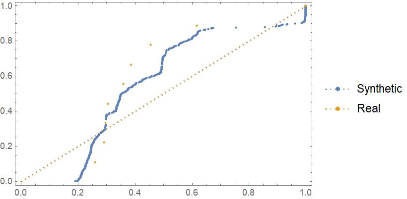
Probability Plot for African Americans in Texas
A Probability Plot Compares the CDF of list against the CDF of a normal distribution.
ProbabilityPlot[{Flatten[
   blackpopsforsyntheticdistricts/totalpopforsyntheticdistricting //
    N], TexasDistrictBlackProportion},
 PlotLegends -> {"Synthetic", "Real"}]
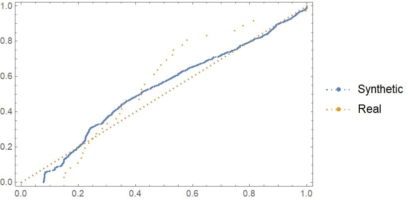
There appears to be a greater deviation in the Texas probability plot than for Massachusetts.
Distribution for Real and Synthetic DIstricts for White People in Texas
Massachusetts
Do the same deviations in patterns apply to a state with a lower African American population percentage?
Histogram[{Flatten[
   Massblackpopsforsyntheticdistricts/
     Masstotalpopforsyntheticdistricting // N],
  MADistrictBlackProportion}, {0, .2, .02}, "PDF",
 ChartLegends -> {"Synthetic", "Real"}]
Unlike Texas, Massachusetts is seen sharing the same distribution for both synthetic and real districts. One simple explanation to this is that in states with low African American populations, there is little reason to gerrymander in respect to race.
Probability Plot for African Americans
A Probability Plot Compares the CDF of list against the CDF of a normal distribution
ProbabilityPlot[{Flatten[
Massblackpopsforsyntheticdistricts/Masstotalpopforsyntheticdistricting //
N], MADistrictBlackProportion}, PlotLegends -> {"Synthetic", "Real"}]
For this histogram, I ran FindGraphPartition successfully 2000 times, creating 7200 different districts.
As one can see, the real districts do a pretty good job following the distribution of synthetic districts.
Conclusion
By incorporating graph theory and data for each tract, I have created a new way of creating and analyzing districts. My partitioning algorithms can create realistic, compact, and continuous districts by taking into account the population of each tract and if the tract is on the border of a county. Furthermore, by comparing synthetic districts to real districts in all states, my code could be used to further analyze districts for gerrymandering, both partisan and racial.


