Simulations of hard circles colliding elastically are fairly common in textbook presentations of event-driven simulation. Even ignoring corner cases such as multiple-disk collisions, it's not entirely easy to write the code. a typical collision involves an angle of incidence and transfer of momentum on two Cartesian dimensions. Stephen Wolfram had the idea of switching out hard spheres for hard squares, which removes the difficulty with angle of incidence and simplifies the equations of momentum transfer. The purpose of this memo is to implement an event-driven algorithm for time-evolving elastic collisions of hard squares trapped in a rigid, immobile container.

[ For instructive purposes, I'm just going to copy and paste from my development notebook with some comments interspersed. At the end we'll need a quality revision to fix some of the hacks that show up along the way. Business as usual, publish in the cloud, etc.]

We will start by defining how the squares move when unconstrained, how their motion changes when they interact with a wall of the container, and how they collide with each other. The massive squares will move through unobstructed space with constant velocity. Squares will be aligned relative to the walls of the rectangular container, so that they meet edge-to-wall when reaching a boundary. Then reflection off a wall reverses the component of the velocity vector normal to the wall. Similarly, when squares meet flat-on edge-to-edge, normal components of their respective velocity vectors will change according to typical high-school formula for collisions in one dimension. Unfortunately, it is somewhat nonphysical that the squares themselves do not rotate, but that is okay for a starter example.

Let's say that we have two squares in a box $[0,15] \times [0,15]$, and they move parallel from one corner to another along a diagonal. We could initialize such a condition as follows:

InitializeCHS[
  phaseSpace_, bounds_
  ] := Association[
  "BoundingBox" -> bounds,
  "ExternalMomentum" -> {0, 0}, "Time" -> 0,
  "PhaseSpace" -> Association[MapThread[
     Rule[#1, Append[#2, "Index" -> #1]] &,
     {Range[Length[phaseSpace]], phaseSpace}]]]

state = InitializeCHS[{
   <|"Position" -> {2, 3}, "Velocity" -> {1, 1}, "Mass" -> 1, 
    "Index" -> 1|>,
   <|"Position" -> {2, 1}, "Velocity" -> {1, 1}, "Mass" -> 1, 
    "Index" -> 2|>
   }, {{0, 15}, {0, 15}}]

Out[]= <|
"BoundingBox" -> {{0, 15}, {0, 15}}, 
"ExternalMomentum" -> {0, 0}, 
"Time" -> 0, 
"PhaseSpace" -> <|
        1 -> <|"Position" -> {2, 3}, "Velocity" -> {1, 1},  "Mass" -> 1, "Index" -> 1|>, 
        2 -> <|"Position" -> {2, 1}, "Velocity" -> {1, 1}, "Mass" -> 1,  "Index" -> 2|>
 |>|>

The requirement of having constant velocities between collisions is very nice. It allows us to calculate exact times when the squares will reflect from walls. If they are on a linear trajectory to collide with each other, we can also calculate the time when they meet edge-to-edge. In the present algorithm, this information gets added to the state vector:

ReflectTime[x1_, 0, bounds_] = Infinity;

ReflectTime[x1_, v1_, bounds_] := Max[
  Divide[2 bounds[[1]] + 1 - 2 x1, 2 v1],
  Divide[2 bounds[[2]] - 1 - 2 x1 , 2 v1]
  ]

AddReflectionTimes[state_] := Module[{statePlus = state},
  statePlus["ReflectionTimes"] = Association[
    Map[{#["Index"]} -> MapThread[ReflectTime,
        {#["Position"], #["Velocity"], state["BoundingBox"]}
        ] &, Values[state["PhaseSpace"]]]];
  statePlus]

CollideTime[_, vx1_, _, vx1_,
  _, _, _, _] := Infinity

CollideTime[
  x1_, vx1_, x2_, vx2_,
  y1_, vy1_, y2_, vy2_] := With[
  {dt = If[Or[
      Abs[x1 - x2] < 1,
      Sign[x1 - x2] == Sign[vx1 - vx2]
      ], -1,
     If[x1 > x2,
      Divide[(x1 - x2) - 1, vx2 - vx1],
      Divide[(x2 - x1) - 1, vx1 - vx2]
      ]]},
  If[And[dt >= 0,
    EuclideanDistance[
      y1 + vy1*dt,
      y2 + vy2*dt
      ] <= 1], dt,
   Infinity
   ]
  ]

AddCollisionTimes[state_] := Module[{statePlus = state},
  statePlus["CollisionTimes"] = Association[
    Map[# -> MapThread[CollideTime,
        Join[#, Reverse /@ #
           ] &[
         Catenate[Map[
           Lookup[#, {"Position", "Velocity"}] &,
           Lookup[state["PhaseSpace"], #]]]]] &,
     Subsets[Keys[state["PhaseSpace"]], {2}]]];
  statePlus]

We don't already have the algorithm pre-packaged, so what we're doing here is basically re-initialization (which means we'll have to re-write the initialization function later):

state2 = AddCollisionTimes[AddReflectionTimes[state]]
Out[] = <|
"BoundingBox" -> {{0, 15}, {0, 15}}, 
 "ExternalMomentum" -> {0, 0}, 
 "Time" -> 0, 
 "PhaseSpace" -> <|
    1 -> <|"Position" -> {2, 3}, "Velocity" -> {1, 1},  "Mass" -> 1, "Index" -> 1|>, 
    2 -> <|"Position" -> {2, 1}, "Velocity" -> {1, 1}, "Mass" -> 1,  "Index" -> 2|>
 |>, 
 "ReflectionTimes" -> <|{1} -> {25/2, 23/2}, {2} -> {25/2, 27/2}|>, 
 "CollisionTimes" -> <|{1, 2} -> {\[Infinity], \[Infinity]}|>|>

We always expect finite reflection times, one each for horizontal and vertical dimensions. But if squares move parallel or away from each other, they can not collide until they go through an event which changes their direction. That explains the appearance of "Infinity" in the collision times.

Once we have a well-prepared state, we can start Iterating through successive states. Just a terminology reminder--by Iterator we mean a Nest-able function whose output is the same type as its input. Every input and output state must have a valid phase space, and a current list of reflection times and collision times. The iterator will then find the next event, propagate masses forward in time, calculate the result of the event, and finally update the list of reflection and collision times. Then we can loop through time as much as we want (unless we happen to hit a corner case with an undetermined configuration).

The propagators are very simple:

PropagateMass[element_Association, time_
  ] := Module[{nextElement = element},
  nextElement["Position"] = Plus[
    nextElement["Position"],
    Times[time, nextElement["Velocity"]]];
  nextElement]

 PropagateState[state_, nextTime_
  ] := Module[{nextState = state},
  Map[Set[nextState["PhaseSpace", #],
     PropagateMass[nextState["PhaseSpace", #], nextTime]
     ] &, Keys[nextState["PhaseSpace"]]];
  Set[nextState["ReflectionTimes"],
   nextState["ReflectionTimes"] - nextTime];
  Set[nextState["CollisionTimes"],
   nextState["CollisionTimes"] - nextTime];
  nextState["Time"] = state["Time"] + nextTime;
  nextState]

And they should be used as follows:

state3 = PropagateState[state2, Min[
   Min[state2["CollisionTimes"]],
   Min[state2["ReflectionTimes"]]
   ]]

Out[] = <|
      "BoundingBox" -> {{0, 15}, {0, 15}}, 
     "ExternalMomentum" -> {0, 0}, 
      "Time" -> 23/2, 
      "PhaseSpace" -> <|
   1 -> <|"Position" -> {27/2, 29/2}, "Velocity" -> {1, 1}, "Mass" -> 1, "Index" -> 1|>, 
   2 -> <|"Position" -> {27/2, 25/2}, "Velocity" -> {1, 1},  "Mass" -> 1, "Index" -> 2|>
 |>, 
 "ReflectionTimes" -> <|{1} -> {1, 0}, {2} -> {1, 2}|>, 
 "CollisionTimes" -> <|{1, 2} -> {\[Infinity], \[Infinity]}|>|>

The masses have moved, but the velocities have not changed. We subtracted some amount off of the reflection and collision times, and next need to look for zeros in these lists (this step could possibly be avoided by better management of the event stack):

FindZeroTimes[eventTimes_
  ] := Association[
  KeyValueMap[Function[{key, val},
    If[SameQ[#, {}], Nothing, key -> #] &[
     MapIndexed[If[PossibleZeroQ[#1],
        #2[[1]], Nothing] &, val]]
    ], eventTimes]]

FindZeroTimes[state3["ReflectionTimes"]]
FindZeroTimes[state3["CollisionTimes"]]

Out[] = <|{1} -> {2}|>
Out[] = <||>

We are working with an overly-simple state, but here is when we really need to worry about the possibility of indeterminate simultaneous collisions. In fact, while I was actually developing this code, I had two or three different states for testing purposes.

For example, on a malicious state, the second output could look as follows:

FindZeroTimes[malState3["CollisionTimes"]]
DuplicateFreeQ[Catenate[%[[All, 1]]]]
Out[] = <|{3, 4} -> {2}, {4, 7} -> {2}, {7, 8} -> {2}, {11, 12} -> {2}, {11, 16} -> {2}, {15, 16} -> {2}|>
Out[] = False

There the False likely indicates a $Failed computation, where we would need to return an error message and stop the computation.

Once we know the list of events from FindZeroTimes, we can resolve collisions or reflections, and return an outgoing state. This part of the code is really the most difficult, and needs to be written line-by-line carefully:

ResolveReflection[element_, inds_
  ] := Module[{nextElement = element},
  Set[nextElement["Velocity"],
   ReplacePart[element["Velocity"],
    # -> -element["Velocity"][[#]] & /@ inds ]];
  nextElement]

ResolveReflections[state_, events_
  ] := Module[{nextState = state, dp},
  dp = Total[KeyValueMap[Function[{key, value},
      ReplacePart[ConstantArray[0, 2],
       Rule[#, Times[2,
           state["PhaseSpace", First[key], "Mass"],
           state["PhaseSpace", First[key], "Velocity"][[#]]
           ]] & /@ value]
      ], events]];
  Set[nextState["ExternalMomentum"],
   Plus[dp, state["ExternalMomentum"]]];
  KeyValueMap[
   Set[nextState["PhaseSpace", First[#1]],
     ResolveReflection[
      state["PhaseSpace", First[#1]],
      #2]] &, events];
  nextState]

ElasticCollision[m1_, m2_, u1_, u2_
  ] := Plus[
  Times[Divide[m1 - m2, m1 + m2], u1],
  Times[Divide[2 m2, m1 + m2], u2]]

ResolveCollision[
  element1_, element2_, inds_
  ] := Module[{nextElement = element1},
  nextElement["Velocity"] = ReplacePart[
    element1["Velocity"],
    Map[Rule[#, ElasticCollision[
        element1["Mass"],
        element2["Mass"],
        element1["Velocity"][[#]],
        element2["Velocity"][[#]]]] &,
     inds]];
  nextElement]

ResolveCollisions[state_, events_
  ] := Module[{nextState = state},
  KeyValueMap[CompoundExpression[
     Set[nextState["PhaseSpace", First[#1]],
      ResolveCollision[
       state["PhaseSpace", First[#1]],
       state["PhaseSpace", Last[#1]],
       #2]],
     Set[nextState["PhaseSpace", Last[#1]],
      ResolveCollision[
       state["PhaseSpace", Last[#1]],
       state["PhaseSpace", First[#1]],
       #2]]
     ] &, events];
  nextState]

Actually, most of this code was copied from a previous implementation and then edited. The second time around it turned out much better! With these functions we can then implement about 90% of the state-to-state iterator:

IterateContinuousHardSquares[state_] := Module[
  {nextTime, nextState, reflections, collisions},
  nextTime = Min[
    Min[state["CollisionTimes"]],
    Min[state["ReflectionTimes"]]
    ];
  nextState = PropagateState[state, nextTime];
  reflections = FindZeroTimes[nextState["ReflectionTimes"]];
  collisions = FindZeroTimes[nextState["CollisionTimes"]];
  If[! Apply[DisjointQ,
     Catenate@*Keys /@ {
       reflections,
       collisions
       }],
   Return[Failure[
     "ReflectionCollision",
     nextState]]
   ];
  If[! DuplicateFreeQ[
     Catenate[Keys[collisions]]],
   Return[Failure[
     "MultipleCollision",
     nextState]]
   ];
  nextState = ResolveReflections[nextState, reflections];
  nextState = ResolveCollisions[nextState, collisions];
  nextState
  ]

All that's left is refreshing reflection and collision times, which can be done by brute force using a similar function to what we have earlier. However this is important. We don't need to update every item. We just need to update items involving squares which have recently gone through an event. At this point the solution and only way forward is obvious:

Quit[]

We have all the code we need to get through iterations, and just need to make minor changes to a few earlier functions. We can scrap what we have above by copy and pasting it into a new notebook, make some quality edits, then upload it to the cloud. Soon it will probably be delivered to WFR, and then much easier to access.

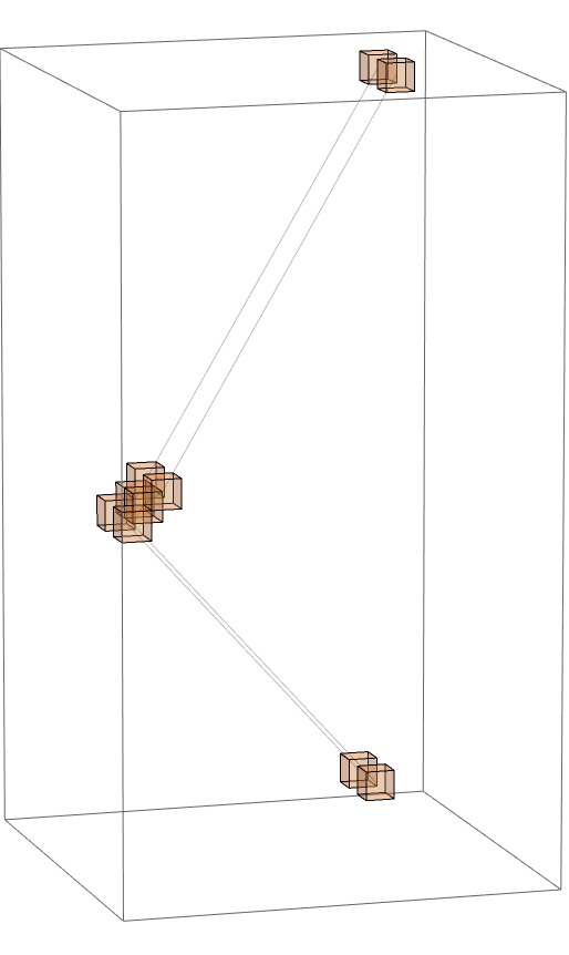
Using the final-draft code we can finally plot the evolution of our simple state, and see that it first reflects, later collides, and generally maintains parallel translation through time:

CHSSpaceTimePlot[
 CHSEventData[{
   <|"Position" -> {2, 3}, "Velocity" -> {1, 1}, "Mass" -> 1, 
    "Index" -> 1|>,
   <|"Position" -> {2, 1}, "Velocity" -> {1, 1}, "Mass" -> 1, 
    "Index" -> 2|>
   }, {{0, 15}, {0, 15}}, 20],
 {{0, 15}, {0, 15}},
 ViewVertical -> {0, 0, 1},
 ViewPoint -> {3, 10, 2}
 ]

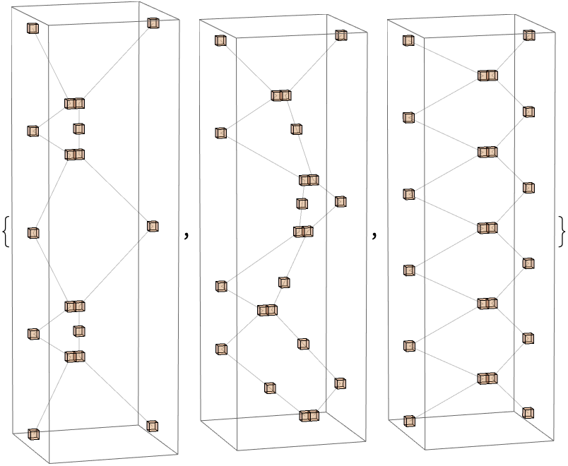
Outputs can be more interesting if we introduce different velocities and masses, even if we set the initial conditions to constrain motion to one dimension (another very simple case):

CHSSpaceTimePlot[
   CHSEventData[
    MakePhaseSpace[
     {{0.5, 7}, {14.5, 7}},
     {{1, 0}, {-#, 0}},
     {2, 1}],
    {{0, 15}, {0, 15}}, 40],
   {{0, 15}, {0, 15}},
   ViewVertical -> {0, 0, 1},
   ViewPoint -> {3, 10, 2},
   SphericalRegion -> False,
   ImageSize -> 120
   ] & /@ {1/2, 1, 2}

These sort of examples are not awe-inspiring, but are easy to check to see that what's happening makes physical sense and obeys conservation laws. We can also generate random initial conditions and plot the event-to-event spacetime evolution:

SeedRandom[3892734];
CHSSpaceTimePlot[
 CHSEventData[
  MakePhaseSpace[
   RandomReal[15, {5, 2}],
   Normalize /@ RandomReal[{-10, 10}, {5, 2}],
   RandomReal[{1, 2}, 5]],
  {{0, 15}, {0, 15}}, 40],
 {{0, 15}, {0, 15}},
 ViewVertical -> {0, 0, 1},
 ViewPoint -> {3, 10, 2},
 SphericalRegion -> False,
 ImageSize -> 400
 ]

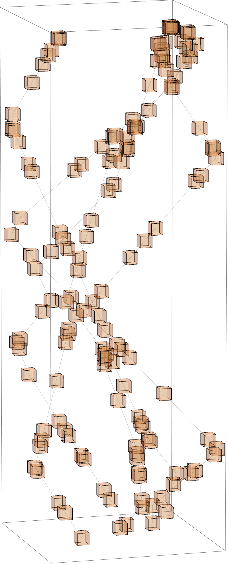
Actually this image gives us a hint that the implementation hasn't reached optimal time, because it isn't exactly a causal graph. We don't really need to calculate the squares at intermediary locations along straight lines between events, but we do anyways. We can probably refine our state update procedure, but what changes need to be made to the state structure? Does each square need to have its own local clock? Perhaps the winter school students will have some good ideas how to refine the code?