Message Boards Message Boards

Some Simple Parameterizations Yielding Visually Stunning Plots

Posted 9 years ago

Some really simple parameterizations yield some elegant-looking results. Some of them are fractal. Here are a few of the coolest I found:

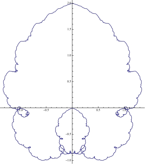
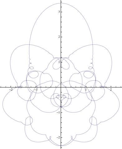
ParametricPlot[Sum[{1/(Sqrt[2])^k Sin[(Sqrt[2])^k t],1/(Sqrt[2])^k Cos[(Sqrt[2])^k t]}, {k, 0, 20}], {t, 0, 1200 Pi}]

enter image description here

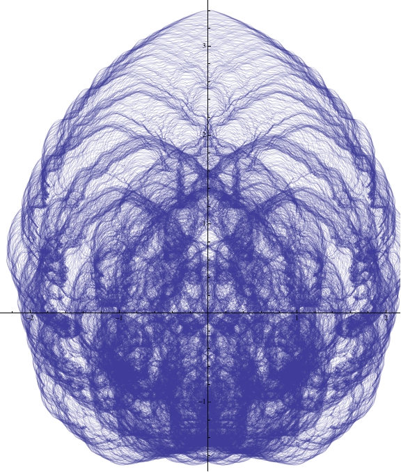
It almost looks photorealistic when we take t and k to large values, a bit like an electron microscope image.

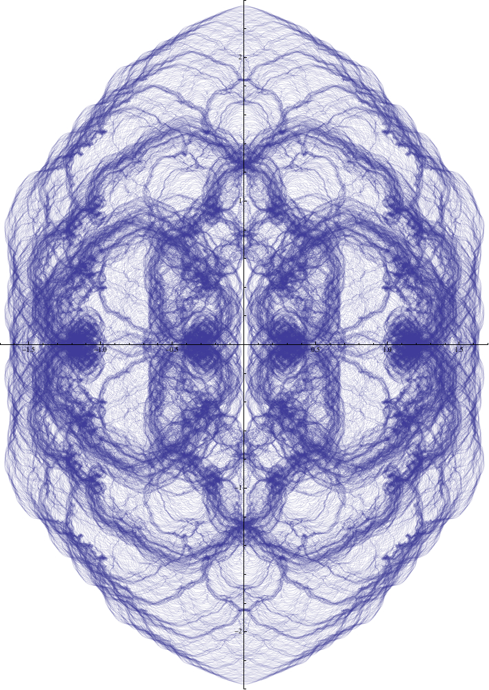
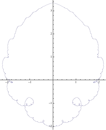
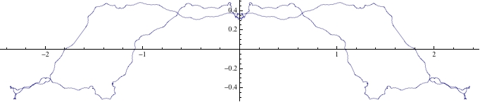
ParametricPlot[Sum[{1/(Sqrt[3])^k Sin[(Sqrt[3])^k t],1/(Sqrt[3])^k Cos[(Sqrt[3])^k t]}, {k, 0, 20}], {t, 0, 1200 Pi}]

enter image description here

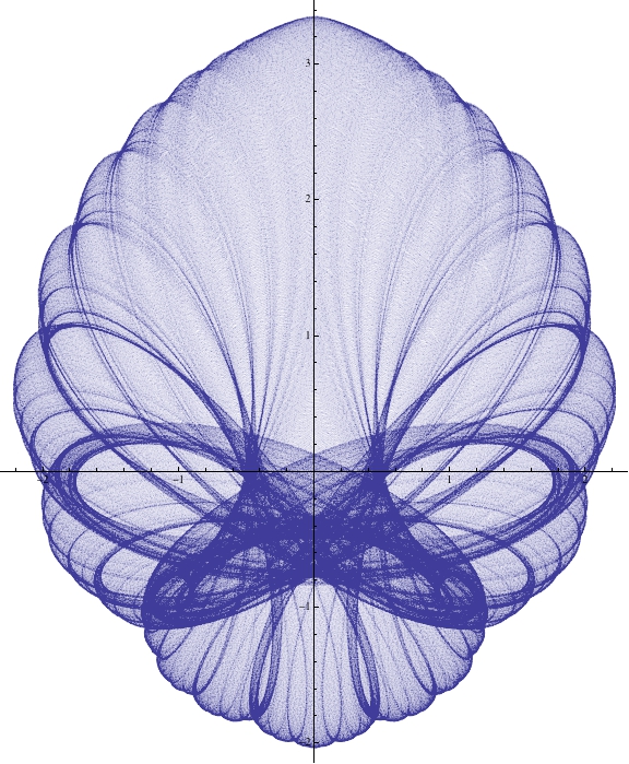
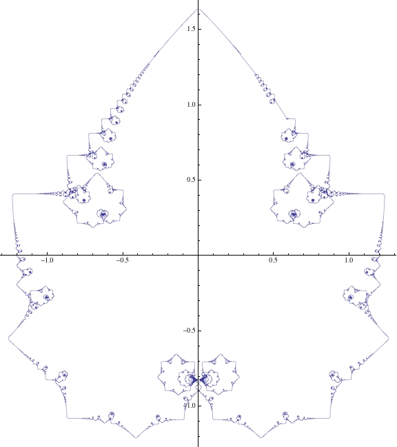
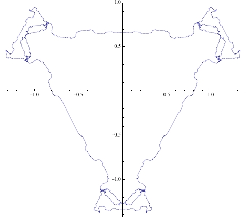
ParametricPlot[Sum[{1/GoldenRatio^k Sin[GoldenRatio^k t],1/GoldenRatio^k Cos[GoldenRatio^k t]}, {k, 0, 20}], {t, 0, 1200 Pi}]

enter image description here

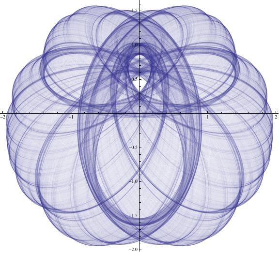
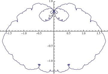
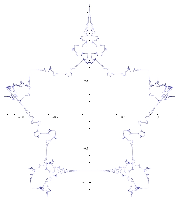
ParametricPlot[Sum[{1/Fibonacci[k] Sin[Fibonacci[k + 13] t],1/Fibonacci[k] Cos[Fibonacci[k + 13] t]}, {k, 1, 20}], {t, 0, 2 Pi}]

enter image description here

ParametricPlot[Sum[{(-1)^k/a^k Sin[a^k t], (-1)^k/a^k Cos[a^k t]}, {k, 0, 20}], {t, 0, 1200 Pi}]

enter image description here

ParametricPlot[Sum[{1/k^2 Sin[k^2 t], 1/k^2 Cos[k^2 t]}, {k, 1, 100}], {t, 0, 2 Pi}]

enter image description here

ParametricPlot[Sum[{1/2^k Sin[2^k t], 1/2^k Cos[2^k t]}, {k, 0, 50}], {t, 0, 2 Pi}]

enter image description here

ParametricPlot[Sum[{1/Fibonacci[k] Sin[Fibonacci[k] t], 1/Fibonacci[k] Cos[Fibonacci[k] t]}, {k, 1, 30}], {t, 0, 2 Pi}]

enter image description here

ParametricPlot[Sum[{(-1)^k/2^k Sin[2^k t], (-1)^k/2^k Cos[2^k t]}, {k, 0, 20}], {t, 0, 2 Pi}]

enter image description here

ParametricPlot[Sum[{1/Fibonacci[k] Sin[k^2 t], 1/Fibonacci[k] Cos[k^2 t]}, {k, 1, 150}], {t, 0, 2 Pi}]

enter image description here

ParametricPlot[Sum[{(-1)^k/k! Sin[(-1)^k k! t], (-1)^k/k! Cos[(-1)^k k! t]}, {k, 0, 100}], {t, 0, 2 Pi}]

enter image description here

ParametricPlot[Sum[{(-1)^k/2^k Sin[(-1)^k 2^k t], (-1)^k/2^k Cos[(-1)^k 2^k t]}, {k, 0, 100}], {t, 0, 2 Pi}]

enter image description here

ParametricPlot[Sum[{(-1)^k/k^2 Sin[(-1)^k k^2 t], (-1)^k/k^2 Cos[(-1)^k k^2 t]}, {k, 1, 100}], {t, 0, 2 Pi}]

enter image description here

ParametricPlot[Sum[{(-1)^k/k^2 Sin[(-1)^k (k - 1)^2 t], (-1)^k/k^2 Cos[(-1)^k (k - 1)^2 t]}, {k, 1, 150}], {t, 0, 2 Pi}]

enter image description here

ParametricPlot[Sum[{1/k^2 Sin[(k - 1)^2 t], 1/k^2 Cos[(k - 1)^2 t]}, {k, 1, 150}], {t, 0, 2 Pi}]

enter image description here

ParametricPlot[Sum[{1/Fibonacci[k] Sin[Fibonacci[k]^2 t], 1/Fibonacci[k] Cos[Fibonacci[k]^2 t]}, {k, 1, 30}], {t, 0, 2 Pi}]

enter image description here

ParametricPlot[Sum[{1/Sqrt[Fibonacci[k]] Sin[Fibonacci[k] t],1/Sqrt[Fibonacci[k]] Cos[Fibonacci[k] t]}, {k, 1, 30}], {t, 0, 2 Pi}]

enter image description here

Please post any similar plots here!

POSTED BY: Bryan Lettner
3 Replies
Posted 9 years ago

Okay so here are two more cool ones:

CurveG[i_] := ParametricPlot[
  Sum[{(-1)^k/GoldenRatio^k Sin[(-1)^k GoldenRatio^k t], (-1)^k/
     GoldenRatio^k Cos[(-1)^k GoldenRatio^k t]}, {k, 0, 40}]
  , {t, (10 i - 10) Pi, 10 i Pi}, PlotStyle -> Thickness[0.0001], 
  MaxRecursion -> 11, ImageSize -> {850, Automatic}]

Show[Table[CurveG[p], {p, 1, 120}]]

enter image description here

Pretty cool, but this next one is my favorite:

CurveJ[i_] := ParametricPlot[
  Sum[{(-1)^k/1.5^k Sin[(-1)^k 1.5^k t], (-1)^k/1.5^
     k Cos[(-1)^k 1.5^k t]}, {k, 0, 30}]
  , {t, (10 i - 10) Pi, 10 i Pi}, PlotStyle -> Thickness[0.00002], 
  MaxRecursion -> 11, PlotRange -> {{-2.5, 2.5}, {-2.5, 2.5}}, 
  ImageSize -> {5000, Automatic}]

Export["HairyStarfish0to6000.jpg", Show[Table[CurveJ[p], {p, 1, 600}]]]
Export["HairyStarfish6000to12000.jpg", Show[Table[CurveJ[p], {p, 600, 1200}]]]
Export["HairyStarfish12000to18000.jpg", Show[Table[CurveJ[p], {p, 1200, 1800}]]]
Export["HairyStarfish18000to24000.jpg", Show[Table[CurveJ[p], {p, 1800, 2400}]]]
Export["HairyStarfish24000to30000.jpg", Show[Table[CurveJ[p], {p, 2400, 3000}]]]
Export["HairyStarfish30000to36000.jpg", Show[Table[CurveJ[p], {p, 3000, 3600}]]]
Export["HairyStarfish36000to42000.jpg", Show[Table[CurveJ[p], {p, 3600, 4200}]]]
Export["HairyStarfish42000to48000.jpg", Show[Table[CurveJ[p], {p, 4200, 4800}]]]
Export["HairyStarfish48000to54000.jpg", Show[Table[CurveJ[p], {p, 4800, 5400}]]]

I did it piecewise like that because it was too taxing on the CPU to go from t=0 to t= large in one go. Each export took about 7 hours. Then I applied some gamma correction (to make lighter and avoid saturation) and stitched them together using ImageMultiply. The plot looks like:

enter image description here

If we look closely, we can see some interesting details beginning to emerge. Almost like a paisley or tribal design. enter image description here

I am going to try it again using a larger image size, a lower value for PlotStyle->Thickness, and taking t all the way to 1,000,000 Pi or so to capture most nuanced detail I can manage. I think with some strategic image processing, we would see some laser-like patterns emerge. On that note, some questions:

-What's the best way to overlay or "add" multiple (10+) images?

-Any general advice on how to enhance the definition and make the patterns "jump out at you"?

I've attached the composite image and some of the constituent images.

Attachments:
POSTED BY: Bryan Lettner

This is great, @Bryan Lettner ! But I cannot reproduce your 1st image from your 1st line of code. How did you get it?

POSTED BY: Sam Carrettie
Posted 9 years ago

Yes, I left out some code for the sake of brevity. Try this:

ParametricPlot[Sum[{1/(Sqrt[2])^k Sin[(Sqrt[2])^k t], 
   1/(Sqrt[2])^k Cos[(Sqrt[2])^k t]}, {k, 0, 15}], {t, 0, 100 Pi}, MaxRecursion -> 10]

Reduced values of t and k, and a high MaxRecursion, should help. Give it about 30-60 seconds to evaluate. With this, you can begin to see the image take shape. However, you will need k > 20 and t > 500Pi to see the details fully emerge, and PlotStyle-> Thickness has to be just right, otherwise it will appear too dark or too faint. I also assembled the plot piecewise, taking t just 10 Pi at a time, because it is very computationally intensive due to high values for t, k, and MaxRecursion. Here is the actual code I used:

CoolCurve[i_] := ParametricPlot[
   Sum[{1/(Sqrt[2])^k Sin[(Sqrt[2])^k t], 1/(Sqrt[2])^k Cos[(Sqrt[2])^k t]}, {k, 0, 20}]
   , {t, (10 i - 10) Pi, 10 i Pi}, PlotStyle -> Thickness[0.0003], MaxRecursion -> 10, ImageSize -> Large];

Export["fhqwhghads.jpg", Show[Table[CoolCurve[n], {n, 0, 120}]]]

It will take at least a couple hours. The image looks a little saturated (too dark)... If I were doing it over again, I would use Thickness[0.0002], and ImageSize->{5000,Automatic} to make a larger, more detailed image. I chose jpg format because .tiff would have been a gigabyte or more. Make sure you have your jpg compression settings to 0.00 to avoid distortion. You can check this by right-clicking any plot, Save Graphic As, choose JPG, click Options, set compression to 0.

Also, if you want to indulge in a little pareidolia for fun, you can see what look like faces along the vertical axis :) . Stay tuned, two more plots coming.

POSTED BY: Bryan Lettner
Reply to this discussion
Community posts can be styled and formatted using the Markdown syntax.
Reply Preview
Attachments
Remove
or Discard

Group Abstract Group Abstract