Message Boards Message Boards

Modeling wind speed distributions with machine learning

What is distribution of wind speed magnitudes at a given geographic location? You could approach this manually like the authors of this paper:

Mixture probability distribution functions to model wind speed distributions

where main conclusion was:

Results show that mixture probability functions are better alternatives to conventional Weibull, two-component mixture Weibull, gamma, and lognormal PDFs to describe wind speed characteristics.

Or you can use Machine Learning and new function FindDistribution. Let's first get a sample of data, say for Boston for recent 5 years:

windBOSTON = WeatherData["Boston", "WindSpeed", {{2010}, {2015}, "Day"}];    
DateListPlot[windBOSTON]

enter image description here

Now get the magnitudes and apply FindDistribution

mags = QuantityMagnitude[windBOSTON["Values"]];
dis = FindDistribution[mags]

which gives, guess what, a MixtureDistribution :

MixtureDistribution[{0.711353, 0.288647}, 
{NormalDistribution[12.8117, 4.74919], LogNormalDistribution[3.06178, 0.308954]}]

Visualizing model versus experimental data looks neat!

Show[
 Histogram[mags, Automatic, "ProbabilityDensity", PlotTheme -> "Detailed"],
 Plot[PDF[dis, x], {x, 0, 50}, PlotRange -> All]]

enter image description here

Try playing with other locations and see what distributions you get. Not always we will get a MixtureDistribution, wind data at different locations can be quite different.

POSTED BY: Vitaliy Kaurov
6 Replies

Hi,

me again... In the paper cited in the first post they study 4 sites/stations, I believe, and they use shorter time series than we do here. As mentioned in my previous post, I want to show the analysis for Europe.

citiesEurope = Flatten[CountryData[#, "LargestCities"] & /@ EntityList[EntityClass["Country", "Europe"]]];
dataEurope = 
  ParallelTable[{citiesEurope[[i]], citiesEurope[[i]]["Coordinates"], FindDistribution[Select[QuantityMagnitude[WeatherData[citiesEurope[[i]], 
 "WindSpeed", {{2004, 1, 1}, Date[], "Day"}]["Values"]], NumberQ]]}, {i, 2, Length[citiesEurope]}];

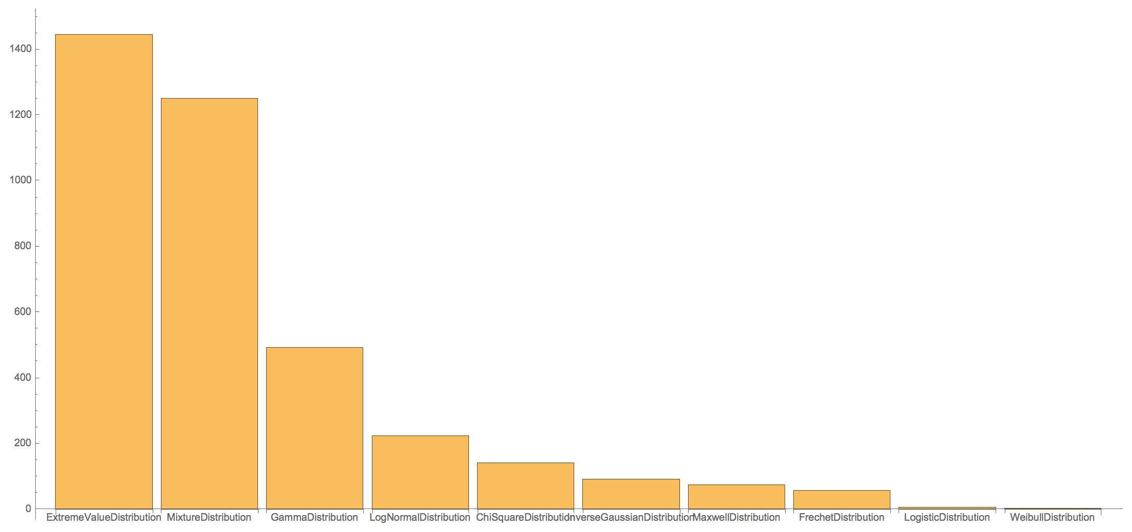
These are the distributions we find:

Tally[Head /@ (DeleteCases[dataEurope[[All, -1]], _FindDistribution])]
(*{{MixtureDistribution, 1251}, {ExtremeValueDistribution, 
  1446}, {FrechetDistribution, 58}, {InverseGaussianDistribution, 
  91}, {LogNormalDistribution, 224}, {GammaDistribution, 
  493}, {ChiSquareDistribution, 142}, {MaxwellDistribution, 
  75}, {WeibullDistribution, 3}, {LogisticDistribution, 6}}*)

The bar chart representation as above can be calculated like so:

BarChart[Apply[Labeled, 
  Reverse[Reverse@SortBy[{{MixtureDistribution, 1251}, {ExtremeValueDistribution, 1446}, {FrechetDistribution, 58}, {InverseGaussianDistribution,91}, {LogNormalDistribution, 224}, {GammaDistribution, 493}, {ChiSquareDistribution, 142}, {MaxwellDistribution, 75}, {WeibullDistribution, 3}, {LogisticDistribution, 6}}, Last], 2], {1}]]
enter image description here

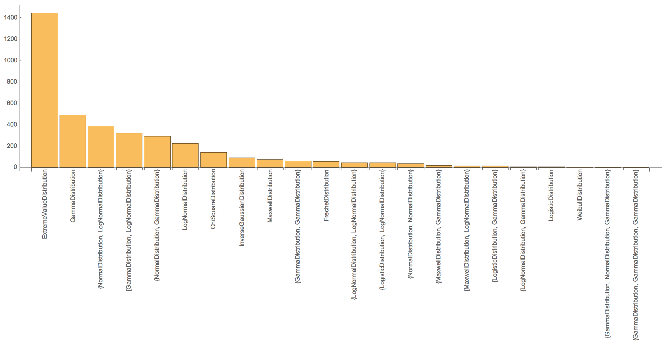
Separating the MixtureDistributions gives:

Reverse@SortBy[Tally[If[Head[#] === MixtureDistribution, Head /@ #[[2]], Head[#]] & /@ DeleteCases[dataEurope[[All, -1]], _FindDistribution]], Last]
(*{{ExtremeValueDistribution, 1446}, {GammaDistribution, 493}, {{NormalDistribution, LogNormalDistribution}, 388}, {{GammaDistribution, LogNormalDistribution}, 322}, {{NormalDistribution, GammaDistribution}, 292}, {LogNormalDistribution, 224}, {ChiSquareDistribution,142}, {InverseGaussianDistribution, 91}, {MaxwellDistribution, 75}, {{GammaDistribution, GammaDistribution}, 59}, {FrechetDistribution, 58}, {{LogNormalDistribution, LogNormalDistribution}, 46}, {{LogisticDistribution, LogNormalDistribution}, 46}, {{NormalDistribution, NormalDistribution}, 37}, {{MaxwellDistribution, GammaDistribution}, 18}, {{MaxwellDistribution, LogNormalDistribution}, 17}, {{LogisticDistribution, GammaDistribution}, 17}, {{LogNormalDistribution, GammaDistribution}, 7}, {LogisticDistribution, 6}, {WeibullDistribution, 3}, {{GammaDistribution, NormalDistribution, GammaDistribution}, 1}, {{GammaDistribution, GammaDistribution, GammaDistribution}, 1}}*)

Here is the BarChart:

BarChart[Apply[Labeled, 
  Reverse[{Rotate[#[[1]], Pi/2], #[[2]]} & /@ Reverse@SortBy[Tally[If[Head[#] === MixtureDistribution, Head /@ #[[2]], Head[#]] & /@ 
  DeleteCases[dataEurope[[All, -1]], _FindDistribution]], Last],2], {1}]]
enter image description here

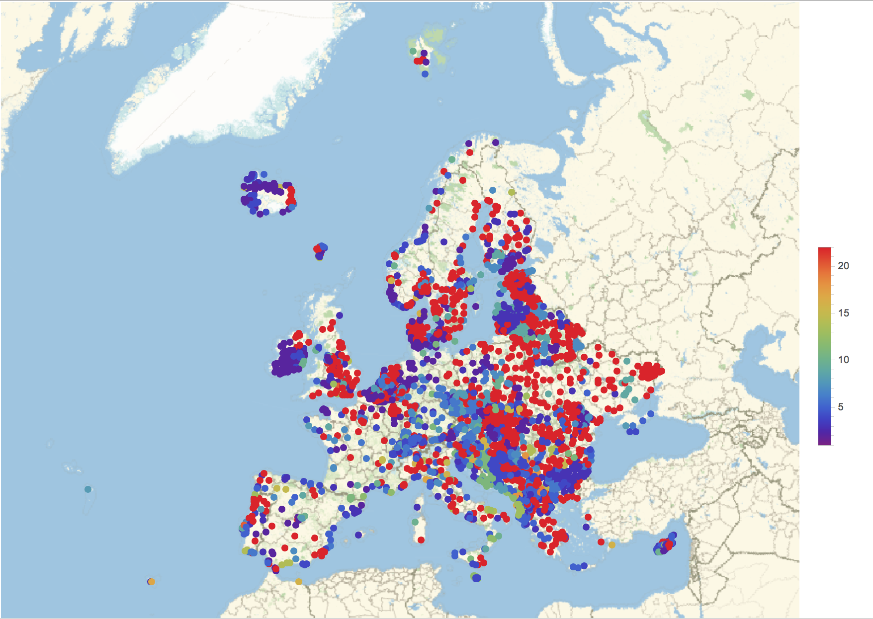
As before we can attach values to the different distributions:

rules = MapThread[Rule, {Reverse@SortBy[Tally[If[Head[#] === MixtureDistribution, Head /@ #[[2]], Head[#]] & /@ 
        DeleteCases[dataEurope[[All, -1]], _FindDistribution]], Last][[All, 1]], Range[Length[Reverse@SortBy[Tally[If[Head[#] === MixtureDistribution, Head /@ #[[2]], Head[#]] & /@ DeleteCases[dataEurope[[All, -1]], _FindDistribution]], Last]]]}]

This is the corresponding plot:

GeoRegionValuePlot[#[[1]] -> #[[2]] & /@ (Transpose[{Select[dataEurope, ! (Head[#[[3]]] === FindDistribution) &][[All, 1]], If[Head[#] === MixtureDistribution, Head /@ #[[2]], Head[#]] & /@ DeleteCases[dataEurope[[All, -1]], _FindDistribution]}] /. rules), ColorFunction -> ColorData["Rainbow"]]
enter image description here

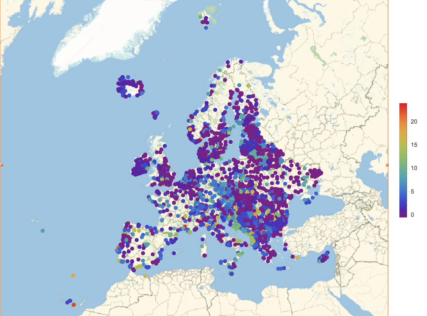
Note that there are too many red dots - they should represent the rare distributions and there should be few. This can be fixed by setting the PlotRange like so:

GeoRegionValuePlot[#[[1]] -> #[[2]] & /@ (Transpose[{Select[dataEurope, ! (Head[#[[3]]] === FindDistribution) &][[All, 1]], If[Head[#] === MixtureDistribution, Head /@ #[[2]], Head[#]] & /@ DeleteCases[dataEurope[[All, -1]], _FindDistribution]}] /. rules), ColorFunction -> ColorData["Rainbow"], PlotRange -> {-0.5, 24}]
enter image description here

This is obviously still very naïve, but it appears that the "distributions are not randomly distributed".

Cheers,

M.

POSTED BY: Marco Thiel

This is amazing idea, @Marco, it makes more sense now. Thanks for sharing! I find it curious, that the Weibull distribution, a popular model for wind, is quite rare and never enters MixtureDistribution. Perhaps because it works better for hourly/ten-minute wind speeds sampling, or at least this is what I understood.

POSTED BY: Vitaliy Kaurov

Nice work! I still think that there might be a seasonal dependence as well in the distributions.

POSTED BY: Kay Herbert

Interesting, but I can't duplicate your answer on my version 10.4:

In[59]:= mags = QuantityMagnitude[windBOSTON["Values"]];
dis = FindDistribution[mags, 2]

Out[60]= {ExtremeValueDistribution[12.6967, 5.66123], 
 MixtureDistribution[{0.680313, 
   0.319687}, {NormalDistribution[13.118, 4.54959], 
   GammaDistribution[7.80677, 2.78237]}]}

or

In[65]:= mags = QuantityMagnitude[windBOSTON["Values"]];
dis = FindDistribution[mags]

Out[66]= ExtremeValueDistribution[12.6967, 5.66123]

on the same data.

I actually was wondering whether the mixture distribution is a consequence of different weather patterns. Like here in Boston we typically have either warm weather coming out the S to SW or the jet stream dipping down from the W to NW. If so, then one distribution would be more prevalent in the winter and another in the summer.

POSTED BY: Kay Herbert

Thanks for pointing this out, @Kay Herbert, indeed the results are different. This is because FindDistribution is constantly getting improved between releases and your result has a higher validity. Strictly speaking these are approximate models and I doubt there is really a way to pinpoint the right analytic distribution. If you look at the details section for FindDistribution they have all sort of properties, including "Score" and "Complexity". These give you insight into their pros and cons when you request more than a single model. And you are right about the right choice of a scale or granularity in your data when you search for a good distribution to describe the patterns specific to your interests.

POSTED BY: Vitaliy Kaurov

Hi Vitaliy,

this is really nice. I had noticed before that FindDistribution suggests different distributions in different places. Here is an example for the UK.

citiesUK = CountryData["UnitedKingdom", "LargestCities"];
data = {#, #["Coordinates"], 
     FindDistribution[
      Select[QuantityMagnitude[
        WeatherData[#, "WindSpeed", {{2004, 1, 1}, Date[], "Day"}][
         "Values"]], NumberQ]]} & /@ citiesUK;
Plot[PDF[#, x] & /@ 
  DeleteCases[data[[All, -1]], _FindDistribution], {x, 0, 50}, 
 AxesLabel -> {"Windspeed", "Probability"}]

enter image description here

It is relatively easy to see what distribution are found with which frequency:

Tally[Head /@ (DeleteCases[data[[All, -1]], _FindDistribution])]
(*{{MixtureDistribution, 15}, {ExtremeValueDistribution, 61}, {GammaDistribution, 20}, {InverseGaussianDistribution, 1}, {WeibullDistribution, 1}, {MaxwellDistribution, 1}}*)

Or

BarChart[Apply[Labeled, Reverse[Reverse@SortBy[{{MixtureDistribution, 15}, {ExtremeValueDistribution, 61}, {GammaDistribution, 20}, {InverseGaussianDistribution, 1}, {WeibullDistribution, 1}, {MaxwellDistribution, 1}}, Last],2], {1}]]

enter image description here

I'd like to study the MixtureDistributions in more detail and read out the constituent parts:

If[Head[#] === MixtureDistribution, Head /@ #[[2]], Head[#]] & /@ DeleteCases[data[[All, -1]], _FindDistribution]

I can tally that now:

Reverse@SortBy[Tally[If[Head[#] === MixtureDistribution, Head /@ #[[2]], Head[#]] & /@ DeleteCases[data[[All, -1]], _FindDistribution]],Last]

enter image description here

BarChart[Apply[Labeled, 
  Reverse[{Rotate[#[[1]], Pi/2], #[[2]]} & /@ 
    Reverse@SortBy[
      Tally[If[Head[#] === MixtureDistribution, Head /@ #[[2]], 
          Head[#]] & /@ 
        DeleteCases[data[[All, -1]], _FindDistribution]], Last], 2], {1}]]

gives

enter image description here

We can now attach values to the different distributions:

rules = MapThread[
  Rule, {Reverse@
    SortBy[Tally[
       If[Head[#] === MixtureDistribution, Head /@ #[[2]], 
          Head[#]] & /@ 
        DeleteCases[data[[All, -1]], _FindDistribution]], Last][[All, 
      1]], Range[
    Length[Reverse@
      SortBy[Tally[
        If[Head[#] === MixtureDistribution, Head /@ #[[2]], 
           Head[#]] & /@ 
         DeleteCases[data[[All, -1]], _FindDistribution]], Last]]]}]

and then plot

GeoRegionValuePlot[#[[1]] -> #[[2]] & /@ 
  Transpose[{Delete[citiesUK, 12], 
    If[Head[#] === MixtureDistribution, Head /@ #[[2]], Head[#]] & /@ 
      DeleteCases[data[[All, -1]], _FindDistribution] /. rules}], 
 GeoRange -> Entity["Country", "UnitedKingdom"], 
 PlotRange -> {-0.5, 11, 0.5}, ColorFunction -> ColorData["Rainbow"]]

enter image description here

These are too few cities to make any general statement, but there might be a pattern to it, i.e. there are three green dots close to Liverpool an Manchester.

I am trying to do this for Europe now, but there are

citiesEurope = Flatten[CountryData[#, "LargestCities"] & /@ EntityList[EntityClass["Country", "Europe"]]];
citiesEurope // Length

3844 cities, so it takes a bit longer.

Cheers,

M.

POSTED BY: Marco Thiel
Reply to this discussion
Community posts can be styled and formatted using the Markdown syntax.
Reply Preview
Attachments
Remove
or Discard

Group Abstract Group Abstract