Hi,
me again... In the paper cited in the first post they study 4 sites/stations, I believe, and they use shorter time series than we do here. As mentioned in my previous post, I want to show the analysis for Europe.
citiesEurope = Flatten[CountryData[#, "LargestCities"] & /@ EntityList[EntityClass["Country", "Europe"]]];
dataEurope =
  ParallelTable[{citiesEurope[[i]], citiesEurope[[i]]["Coordinates"], FindDistribution[Select[QuantityMagnitude[WeatherData[citiesEurope[[i]],
 "WindSpeed", {{2004, 1, 1}, Date[], "Day"}]["Values"]], NumberQ]]}, {i, 2, Length[citiesEurope]}];
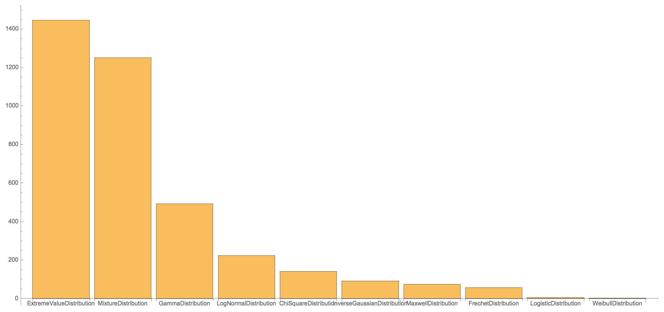
These are the distributions we find:
Tally[Head /@ (DeleteCases[dataEurope[[All, -1]], _FindDistribution])]
(*{{MixtureDistribution, 1251}, {ExtremeValueDistribution,
  1446}, {FrechetDistribution, 58}, {InverseGaussianDistribution,
  91}, {LogNormalDistribution, 224}, {GammaDistribution,
  493}, {ChiSquareDistribution, 142}, {MaxwellDistribution,
  75}, {WeibullDistribution, 3}, {LogisticDistribution, 6}}*)
The bar chart representation as above can be calculated like so:
BarChart[Apply[Labeled,
  Reverse[Reverse@SortBy[{{MixtureDistribution, 1251}, {ExtremeValueDistribution, 1446}, {FrechetDistribution, 58}, {InverseGaussianDistribution,91}, {LogNormalDistribution, 224}, {GammaDistribution, 493}, {ChiSquareDistribution, 142}, {MaxwellDistribution, 75}, {WeibullDistribution, 3}, {LogisticDistribution, 6}}, Last], 2], {1}]]
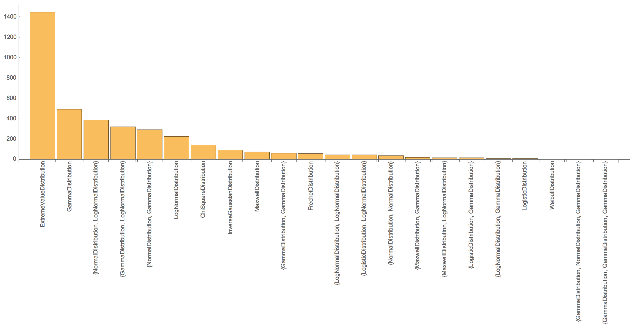
Separating the MixtureDistributions gives:
Reverse@SortBy[Tally[If[Head[#] === MixtureDistribution, Head /@ #[[2]], Head[#]] & /@ DeleteCases[dataEurope[[All, -1]], _FindDistribution]], Last]
(*{{ExtremeValueDistribution, 1446}, {GammaDistribution, 493}, {{NormalDistribution, LogNormalDistribution}, 388}, {{GammaDistribution, LogNormalDistribution}, 322}, {{NormalDistribution, GammaDistribution}, 292}, {LogNormalDistribution, 224}, {ChiSquareDistribution,142}, {InverseGaussianDistribution, 91}, {MaxwellDistribution, 75}, {{GammaDistribution, GammaDistribution}, 59}, {FrechetDistribution, 58}, {{LogNormalDistribution, LogNormalDistribution}, 46}, {{LogisticDistribution, LogNormalDistribution}, 46}, {{NormalDistribution, NormalDistribution}, 37}, {{MaxwellDistribution, GammaDistribution}, 18}, {{MaxwellDistribution, LogNormalDistribution}, 17}, {{LogisticDistribution, GammaDistribution}, 17}, {{LogNormalDistribution, GammaDistribution}, 7}, {LogisticDistribution, 6}, {WeibullDistribution, 3}, {{GammaDistribution, NormalDistribution, GammaDistribution}, 1}, {{GammaDistribution, GammaDistribution, GammaDistribution}, 1}}*)
Here is the BarChart:
BarChart[Apply[Labeled,
  Reverse[{Rotate[#[[1]], Pi/2], #[[2]]} & /@ Reverse@SortBy[Tally[If[Head[#] === MixtureDistribution, Head /@ #[[2]], Head[#]] & /@
  DeleteCases[dataEurope[[All, -1]], _FindDistribution]], Last],2], {1}]]
As before we can attach values to the different distributions:
rules = MapThread[Rule, {Reverse@SortBy[Tally[If[Head[#] === MixtureDistribution, Head /@ #[[2]], Head[#]] & /@
        DeleteCases[dataEurope[[All, -1]], _FindDistribution]], Last][[All, 1]], Range[Length[Reverse@SortBy[Tally[If[Head[#] === MixtureDistribution, Head /@ #[[2]], Head[#]] & /@ DeleteCases[dataEurope[[All, -1]], _FindDistribution]], Last]]]}]
This is the corresponding plot:
GeoRegionValuePlot[#[[1]] -> #[[2]] & /@ (Transpose[{Select[dataEurope, ! (Head[#[[3]]] === FindDistribution) &][[All, 1]], If[Head[#] === MixtureDistribution, Head /@ #[[2]], Head[#]] & /@ DeleteCases[dataEurope[[All, -1]], _FindDistribution]}] /. rules), ColorFunction -> ColorData["Rainbow"]]
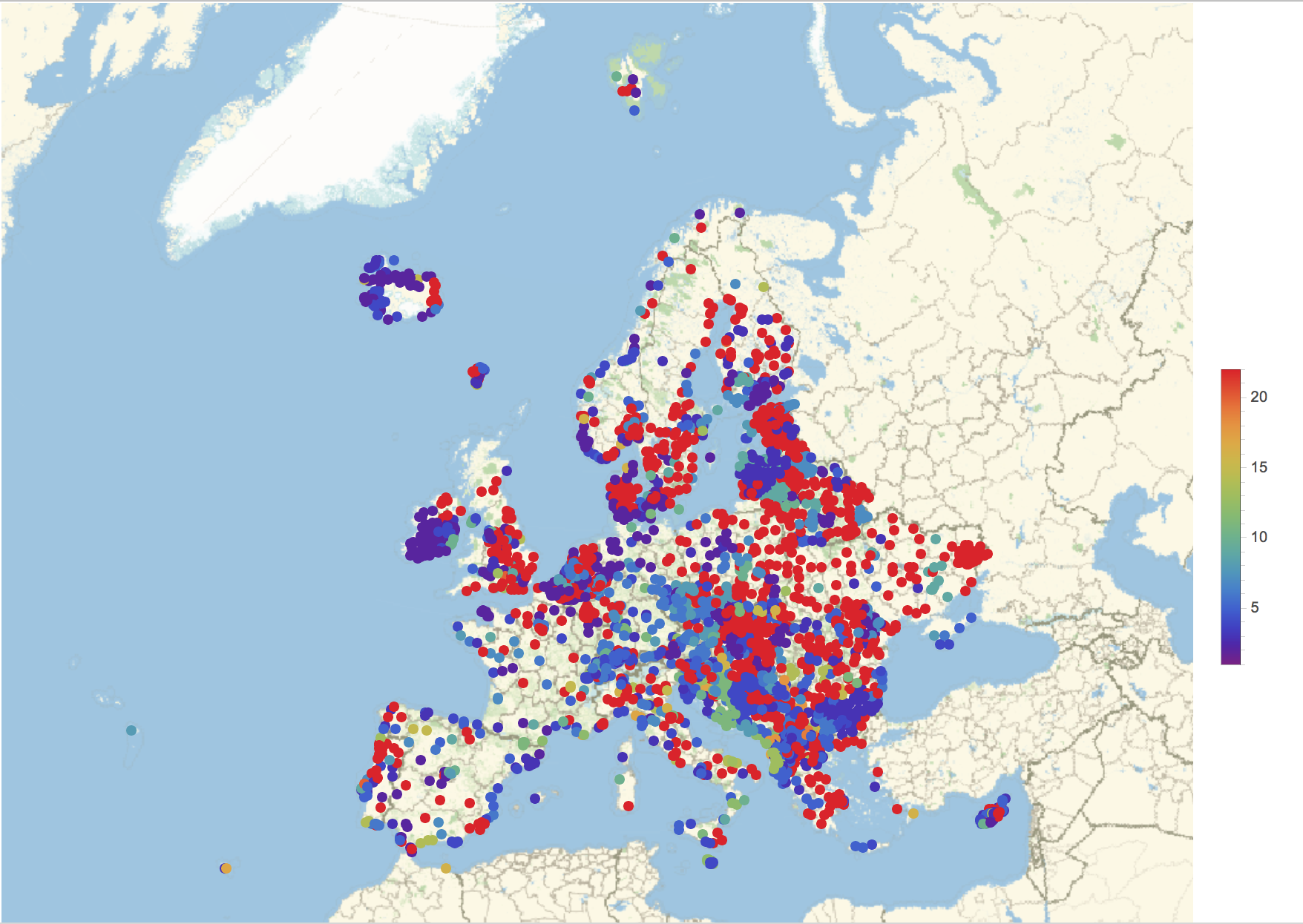
Note that there are too many red dots - they should represent the rare distributions and there should be few. This can be fixed by setting the PlotRange like so:
GeoRegionValuePlot[#[[1]] -> #[[2]] & /@ (Transpose[{Select[dataEurope, ! (Head[#[[3]]] === FindDistribution) &][[All, 1]], If[Head[#] === MixtureDistribution, Head /@ #[[2]], Head[#]] & /@ DeleteCases[dataEurope[[All, -1]], _FindDistribution]}] /. rules), ColorFunction -> ColorData["Rainbow"], PlotRange -> {-0.5, 24}]
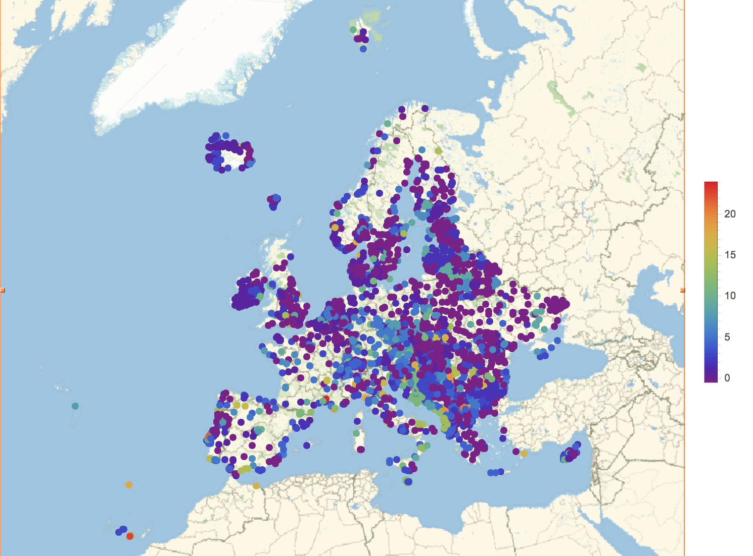
This is obviously still very naïve, but it appears that the "distributions are not randomly distributed".
Cheers,
M.


