Message Boards Message Boards

Plot a torus knot with ParametricPlot3D?

Posted 7 years ago

Hello everyone, I hope you can explain why I am getting an empty graphic, I happen to be taking the code that Paul Nylander shares on his web page, and when I run it in mathematica I do not get any graphics, here I share a screenshot so that understand my problem better,

graphic obtained

I think the problem is in how it uses ParametricPlot3D, but I hope someone who knows the reason, please explain, thanks in advance.

Image and code from Paul`s page

how make it

Code used for me, this is

normalize[x_] := x/Sqrt[x.x]; 
p[t_] := {(1 + 0.3 Cos[11 t/3]) Cos[t], (1 + 0.3 Cos[11 t/3]) Sin[t], 
  0.3 Sin[11 t/3]};
f[t_, theta_] := 
  Module[{dp = p'[t], ddp = p''[t], tangent, normal1, normal2}, 
   tangent = normalize[dp]; 
   normal1 = normalize[ddp (dp.dp) - dp (dp.ddp)]; 
   normal2 = Cross[tangent, normal1]; 
   p[t] + 0.1 (normal1 Cos[theta] + normal2 Sin[theta])];

ParametricPlot3D[
 Append[f[t, theta], {EdgeForm[], SurfaceColor[Hue[t/(2 Pi)]]}], {t, 
  0, 6 Pi}, {theta, 0, 2 Pi}, PlotPoints -> {360, 15}, 
 Compiled -> False]
POSTED BY: Luis Ledesma
2 Replies
Posted 7 years ago

Thank you very much for your great help Sander now if you get the graph that I thought, I kept browsing Paul's page and I'm interested in the following image, 
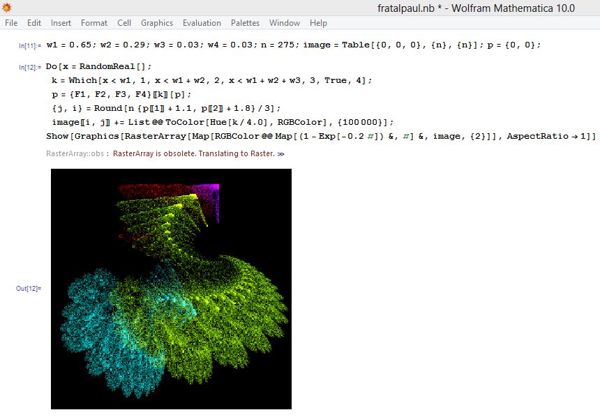
But now it turns out that you get another error message related to Raster Array, I share the image so you have an idea of what I am talking about, when switching from RasterArray to Raster I get an empty graph again. To conclude I would like to tell you that Paul used version 4 of Mathematica that is why it changes the commands considerably. Saludos y gracias amigo.

RasterArray

V1[{x_, y_}] := {Sin[x], Sin[y]};
F1[p_] := Module[{p2 = {{0.81, -0.33}, {0.08, 0.89}}.p + {0.24, -0.07}}, 0.88p2 + 0.12V1[p2]];
F2[p_] := Module[{p2 = {{0.3, 0.52}, {-0.56, 0.37}}.p + {-0.09, -0.42}}, 0.88p2 + 0.12V1[p2]];
F3[p_] := V1[{{-0.43, 0.38}, {-0.2, -0.44}}.p + {1.74, 1.21}];
F4[p_] := V1[{{-0.49, -0.27}, {0.28, -0.53}}.p + {0.51, 0.62}];
w1 = 0.65; w2 = 0.29; w3 = 0.03; w4 = 0.03;
n = 275; image = Table[{0, 0, 0}, {n}, {n}]; p = {0, 0};
Do[x = Random[]; k = Which[x < w1, 1, x < w1 + w2, 2, x < w1 + w2 + w3, 3, True, 4]; p = {F1, F2, F3, F4}[[k]][p]; {j,i} = Round[n{p[[1]] + 1.1, p[[2]] + 1.8}/3]; image[[i, j]] += List @@ ToColor[Hue[k/4.0], RGBColor], {100000}];
Show[Graphics[RasterArray[Map[RGBColor @@ Map[(1 - Exp[-0.2#]) &, #] &, image, {2}]], AspectRatio -> 1]]
POSTED BY: Luis Ledesma

Here is the correct one:

p[t_]:={(1+0.3 Cos[11 t/3]) Cos[t],(1+0.3 Cos[11 t/3]) Sin[t],0.3 Sin[11 t/3]};
f[t_,theta_]:=Module[{dp=p'[t],ddp=p''[t],tangent,normal1,normal2},
    tangent=Normalize[dp];
    normal1=Normalize[ddp (dp.dp)-dp (dp.ddp)];
    normal2=Cross[tangent,normal1];
    p[t]+0.1 (normal1 Cos[theta]+normal2 Sin[theta])
];

ParametricPlot3D[f[t,theta],{t,0,6 Pi},{theta,0,2 Pi},ColorFunction->Function[{x,y,z,u,v},Hue[u]],PlotPoints->{160, 20},MaxRecursion->0]

You can't specify the surface color like the website does, perhaps in a VERY old version it was possible. I can't remember that though... You have to use ColorFunction. Note that Normalize is available in the Wolfram Language. Speed can be improved by not repeating the differentiation each time...

POSTED BY: Sander Huisman
Reply to this discussion
Community posts can be styled and formatted using the Markdown syntax.
Reply Preview
Attachments
Remove
or Discard

Group Abstract Group Abstract